


Abstract
We have analysed the Fermi Large Area Telescope (LAT) data on the SNR G73.9+0.9. We have confirmed a previous detection of high-energy γ-rays from this source at a high significance of ≃12σ. The observed spectrum shows a significant curvature, peaking in EFE at ∼1 GeV. We have also calculated the flux upper limits in the mm-wavelength and X-ray ranges from Planck and XMM–Newton, respectively. We have inspected the intensity of the CO (1→0) emission line and found a large peak at a velocity range corresponding to the previously estimated source distance of ∼4 kpc, which may indicate an association between a molecular cloud and the supernova remnant (SNR). The γ-ray emission appears due to interaction of accelerated particles within the SNR with the matter of the cloud. The most likely radiative process responsible for the γ-ray emission is decay of neutral pions produced in ion–ion collisions. While a dominant leptonic origin of this emission can be ruled out, the relativistic electron population related to the observed radio flux will necessarily lead to a certain level of bremsstrahlung γ-ray emission. Based on this broad-band modelling, we have developed a method to estimate the magnetic field, yielding B ≳ 80 μG at our best estimate of the molecular cloud density (or less at a lower density). G73.9+0.9 appears similar, though somewhat weaker, to other SNRs interacting with a local dense medium detected by the LAT.
1 INTRODUCTION
G73.9+0.9 is a supernova remnant (SNR) located in the Cygnus arm of the Galaxy. It was first observed and identified as an SNR in radio in the Effelsberg Galactic Plane survey (Reich et al. 1986). High-resolution imaging at 1.42 GHz (see Kothes et al. 2006 and references therein) shows a morphology consisting of a shell-like feature to the south with a sharp outer boundary and a centrally peaked diffuse emission to the east.
The radio emission has the total flux of ∼8 Jy at 1.4 GHz and the energy index of α ≃ −0.23 (Fν ∝ να; measured between 0.4 and 10 GHz), corresponding to the photon index of Γ = 1.23 (Fν ∝ ν1−Γ). Lorimer, Lyne & Camilo (1998) searched for pulsed emission from the centre of the shell using the 76-m Lovell radio telescope, but without success.
The region towards the source has been observed by the Planck mission1 (Tauber et al. 2010; Planck Collaboration I 2015a), but since G73.9+0.9 lies in a rather complex region of the Galactic plane, no results have been reported. Here, we obtain upper limits in the 30–143 GHz range, see Section 2.1.
Optical line diffuse emission has been observed towards the direction of this SNR (Lozinskaya, Sitnik & Pravdikova 1993; Mavromatakis 2003). The optical spectrum implies an electron density of ne ≲ 50 cm−3 at some locations within the SNR, and a moderate shock velocity of vsh ≲ 90 km s−1. These observations have allowed an estimate of the age of the SNR to be T ∼ 11–12 kyr. Its distance has been variously estimated. The most recent determination of Pavlović et al. (2013) puts it D = 4.0 kpc, based on the radio surface brightness to diameter relation. The radial velocity of G73.9+0.9 has been measured by Lozinskaya et al. (1993) as 4 ± 3 km s−1.
The SNR has not been detected in X-rays. We obtain an upper limit from XMM–Newton, see Section 2.1. The region has also been observed with Imaging Cherenkov Telescopes at very high energies, but no signal has been found. In particular, it was covered as part of the HEGRA Galactic Plane survey (Aharonian et al. 2002). The 2-h exposure resulted in an upper limit on the number flux of N(>E) < 3.15 × 10⁻¹²(E/1 TeV)−1.59 cm−2 s−1 (Aharonian et al. 2002). The VERITAS array also observed this region; the preliminary upper limit at the location of the SNR is |$N(>\!300\,{\rm GeV})\lesssim 2.3\times 10^{-12}\, \mathrm{cm}^{-2} \,\mathrm{s}^{-1}$| (Theling 2009).
At high-energy γ-rays (0.1 GeV ≲ E ≲ 100 GeV), Malyshev, Zdziarski & Chernyakova (2013) have reported a detection of γ-ray emission from the direction of G73.9+0.9 using the Large Area Telescope (LAT) on board of Fermi. The γ-ray emission was discovered when investigating the region around Cyg X-1, which lies 3|$_{.}^{\circ}$|2 away of G73.9+0.9. The γ-ray source was detected with the test statistic (Ts; Mattox et al. 1996) of ≃50, at RA 303.42, Dec. 36.21, which is only ∼10 arcmin away from the catalogue position of the remnant, at RA 303.404 (20 13 37), Dec. 36.115 (36 06 54.0), corresponding to the Galactic coordinates of l = 73.77, b = 0.94. This detection has recently been confirmed in the Fermi-Large Area Telescope Third Source Catalogue (3FGL; Fermi-LAT Collaboration 2015), as the source named J2014.4+3606 with the significance2 of 4.5σ. Here, we re-analyse a significantly larger data set with the present instrumental calibration, and obtain significantly better statistical results.
We present here a dedicated analysis of the currently available data set obtained with the LAT on the SNR and an investigation of the molecular content around it, derived from an analysis of the CO line (1→0) intensity at 115 GHz (2.6 mm) in the region, observed with the CfA telescope (Dame et al. 1987). We also study models possibly explaining the multiwavelength spectrum of G73.9+0.9.
2 MULTIWAVELENGTH DATA ANALYSIS AND RESULTS
2.1 The imaging and spectral analysis
We have analysed the Fermi LAT data derived from a 15° radius region centred on the position of G73.9+0.9. Almost seven years of data obtained during MJD 54682–57209 (2008 August 04–2015 July 06) were processed using the LAT standard tools (software version v10r0p5), and analysed with the P8R2 response functions (SOURCE class photons). We have applied the standard cleaning to suppress the effect of the Earth albedo background, excluding time intervals when the Earth was in the field of view (FoV; when its centre was |${>}52\circ$| from the zenith), and those in which a part of the FoV was observed with the zenith angle |${>}90\circ$|.
We have selected events with energies between 0.1 GeV to 300 GeV, performing binned likelihood analysis. It is based on the fitting of a model of diffuse and point source emission within selected region to the data. The spatial model includes diffuse Galactic and extragalactic backgrounds (gll_iem_v06.fits and iso_P8R2_SOURCE_V6_v06.txt templates) and the sources from the 3FGL catalogue. We split the whole energy range into narrow energy bins, performing the fitting procedure in each bin separately. In each bin, the spectral shapes of all sources are assumed to be power laws with Γ = 2. The spectral shapes of diffuse Galactic and extragalactic backgrounds are given by the corresponding templates. The normalizations of the fluxes of all sources and the diffuse background are treated as free parameters during the fitting. The analysis is performed with the python tools.3 The upper limits are calculated with the UpperLimits module provided with the Fermi/LAT software and correspond to the 95 per cent (≃2.5σ) false-chance probability.
We localize the position of G73.9+0.9 by building the Ts map of the selected region. The colour image in Fig. 1 shows this map, which illustrates the significance of adding a point source to the model of the region, which follows the χ2 distribution and is approximately |${\simeq }\! \sqrt{T_{\rm s}}$| (Mattox et al. 1996). The model in this case includes all the sources described above, except 3FGL J2014.4+3606, which corresponds to G73.9+0.9 in the 3FGL catalogue. We see a clear γ-ray excess at the position of G73.9+0.9 in the 1–3 GeV energy band. The centroid of the image is the same as that in the 3FGL catalogue. The source shows a point-like morphology, with the 3σ upper limit on its radius (corresponding to the decrease of Ts by 9 for the uniform-brightness disc model with respect to the point-source model) of 0|$_{.}^{\circ}$|23 in the 0.3–3 GeV energy band. The maximum of the Ts for the γ-ray source lies 0|$_{.}^{\circ}$|1 from the centre of the radio emission from G73.9+0.9, which offset is not statistically significant. This is also shown in Fig. 1, where the black contours show the 4.85 GHz continuum emission from the GB6/PMN survey (Condon et al. 1994).
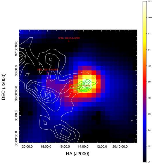
The colour image shows the Ts map of the region in 0.3–3 GeV energy band with 0|$_{.}^{\circ}$|1 × 0|$_{.}^{\circ}$|1 pixels. All sources except 3FGL J2014.4+3606 (G73.9+0.9) were included into the region model and thus are not present on the map; |$\sqrt{T_{\rm s}}$| gives the significance of a point-like source added to the model at a selected point. The green contours show the image of the SNR in 4.85 GHz continuum emission (Condon et al. 1994). The white contours are derived from the intensity data of the 115 GHz CO line (1→0; Dame et al. 2001) in the 1–7 km s−1 velocity range.
The energy spectrum for a point-like source centred at the position of G73.9+0.9 was derived by means of the binned likelihood fitting, as described above. We show it in Fig. 2. The shown error bars correspond to 1σ statistical errors. In the energy range of 0.1–300 GeV the spectrum can be fitted with a power law, which we show in Fig. 2, with the photon index of Γ = 2.73 ± 0.13 and the normalization of N0 = (2.17 ± 1.10) × 10−11 erg cm−2 s−1, defined as the value of EFE at 0.1 GeV. This fit yields the Ts ≃ 64, which corresponds to σ ≃ 7.7. This confirms, at a higher significance, the presence of this source in γ-rays discovered by Malyshev et al. (2013).
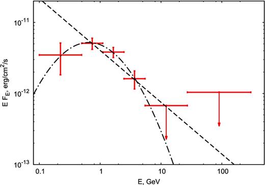
The γ-ray spectrum of the point-like source at the position of G73.9+0.9. The shown error bars present 1σ statistical uncertainties and the upper limits correspond to 95 per cent confidence (about 2.5σ). The dashed and dot–dashed curves shows the best-fitting power-law and lognormal spectrum, respectively.
However, the spectral points show a clear curvature in the spectrum, with the peak around 1 GeV. We confirm the high statistical significance of the presence of a curvature by fitting a lognormal model (see Appendix A) to the 0.1–300 GeV photon-energy band, which yields a much higher Ts ≃ 150, which corresponds to the significance of ≃11.8σ (with an addition of one free parameter with respect to the power-law fit). The fit parameters are N0 = (7.7 ± 1.0) × 10−12 cm−2 s−1 MeV−1 (defined as in equation A2), Eb = 0.65 ± 0.04 GeV, which is the peak of the lognormal distribution in EFE, and β = 0.89 ± 0.07. We also obtain a similar Ts for a broken power-law fit, which has two more parameters than a single power law. We have also fitted the spectrum at E ≥ 1 GeV by a power law, to facilitate comparison with Fermi review papers, which give that index for other SNRs, see, e.g. Brandt et al. (2015). We have obtained Γ = 3.2 ± 0.2 and the normalization of N0 = (6.2 ± 0.8) × 10−12 erg cm−2 s−1, given as EFE at 1 GeV.
The integrated 1–100 GeV photon and energy fluxes derived directly from the obtained spectrum (i.e. treating the upper limits as zero-points with the uncertainty treated as a systematic error) are |${\simeq } 2.0^{+1.9}_{-0.24} \times 10^{-9}$| cm−2 s−1 and |${\simeq } 5.2^{+5.0}_{-0.65} \times 10^{-12}$| erg cm−2 s−1, respectively. The estimated γ-ray luminosities for the 0.1–100, 0.5–100 and 1–100 GeV ranges are, respectively, |$28.3^{+9.9}_{-5.9}$|, |$16.4^{+5.7}_{-1.9}$|, and |$9.9^{+6.7}_{-1.2} \times (D/4\,{\rm kpc})^2 \times 10^{33}$| erg s−1.
We have also searched for X-ray emission based on the XMM–Newton pointed observation of the field of G73.9+0.9 on 2006 April 19 (ObsID 0301880601, full window mode, PI: O. Kargaltsev). The observation yields an upper limit of ≲ 2.7 × 10− 14 erg cm−2 s−1 in the energy range of 0.5–4.5 keV within a circle of 90 arcsec radius around the observation pointing of RA 303.48, Dec. 36.25. The analysis has been done using the XMM–Newton online upper-limit software.4 The upper limit is from the MOS2 detector, for which the exposure time is 2550 s; the MOS1 and PN have much shorter exposures. From XMM–Newton and other X-ray observatories, there are no bright X-ray sources seen within the radius of 0|$_{.}^{\circ}$|2 around the SNR centre. From the image of the source in radio at 1.42 GHz (Kothes et al. 2006), we have visually estimated the area of the peak of the SNR emission to be ∼(0|$_{.}^{\circ}$|1)2. This yields an upper limit on the SNR emission within 0.5–4.5 keV of <1.4 × 10⁻¹³ erg cm−2 s−1. This corresponds to EFE < 6.2 × 10⁻¹⁴ erg cm−2 s−1 (assuming Γ = 2), shown in Fig. 3. This upper limit has a systematic uncertainty related to the uncertain source area and the spectral slope, which we roughly estimate to be of a factor of 3.
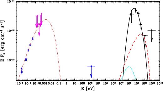
The observed broad-band spectrum of G73.9+0.9. The black symbols with open circles give our γ-ray measurements and upper limits, and the magenta symbols give our upper limits from Planck. The radio data from Kothes et al. (2006) and the upper limit from XMM–Newton are shown by blue crosses and error bars, and by the blue upper limit with an open circle, respectively. The spectrum from decay of neutral pions in the hadronic model is shown by the black solid curve, see Section 2.3. The cyan dot–dashed curve shows the bremsstrahlung emission of e± from decay of charged pions in the same model assuming the SNR age of 12 kyr and at ne = 30 cm−3 and B = 80 μG. The corresponding synchrotron emission is below the shown range of fluxes. The radio spectrum is modelled by synchrotron emission (shown by the red dotted curve) from e-folded power-law electrons with the minimum value of |$B\gamma _0^2$| allowed by the radio data not showing any high-energy cut-off. The normalization of the spectrum yields KeB(1 + p)/2/(4πD2). The red dashed curve shows the maximum bremsstrahlung emission from the same electrons allowed by the data, which implies that B ≳ 80 μG. See Section 2.4 for details.
We have also searched for mm-wavelength emission using the Planck 2015 data (Planck Collaboration VI 2015b; Planck Collaboration VIII 2015c). The source does not appear in the Second Planck Catalogue of Compact Sources (Planck Collaboration XXVI 2015d). We have obtained 2σ upper limits in the 30–143 GHz frequency range using the 2015 full mission maps, and we show them in Fig. 3.
The flux density of the source and the uncertainties used to calculate the upper limits have been measured as follows. For the flux density, aperture photometry centred at the position of the source has been used using an aperture with a radius equal to 1 full width at half-maximum (FWHM). The flux densities have been corrected to take into account that a fraction of the beam solid angle falls outside the aperture. For the rms, we have used an annulus with the inner radius of 1 FWHM and the outer radius of 2 FWHM. For all the frequencies, the FWHMs are the effective beams as listed in column 3 of table 2 of Planck Collaboration XXVI (2015d).
2.2 A molecular cloud around G73.9+0.9
Several GeV-bright SNRs have been shown to interact with colocated molecular clouds. The presence of such a cloud appears to be required for emission of γ-rays detectable by the LAT from old SNRs (Hewitt et al. 2013). A safe identification of interaction with such high-density material would be a detection of masers (see e.g. W51C; Green et al. 2006). A search in the direction of G73.9+0.9 for both OH and H2O masers, at 1.72 GHz and 22 GHz, respectively, gave no results (Woodall & Gray 2007; Hewitt & Yusef-Zadeh 2009). Data from the I-GALFA H i 21-cm line survey did not show any significant excess emission that can be associated with the remnant (Park et al. 2013).
We have calculated the absolute value of the molecular mass using the conversion factor estimated by Dame et al. (2001), XCO = 1.8 × 1020 cm−2(K km/s)−1. Studies of the estimation of the gas content using different tracers show compatible average results (Pedaletti et al. 2015).
We have found that the velocity distribution of the CO content shows a clear excess in the range of velocity of (−2.0, 3.2) km s−1. This overlaps with the velocity range measurement of v ≃ 1–7 km s−1 of Lozinskaya et al. (1993). Thus, we adopt the range of v ≃ 1.0–3.2 km s−1 as the SNR systemic velocity. Based on it and using the Galactocentric rotation–distance relation of Clemens (1985), we estimate the distance of G73.9+0.9 of either 0.2–0.5 kpc or 4.3–4.5 kpc. These estimates bear some systematic uncertainties due to the uncertainty of the rotation curve of Clemens (1985) and to the possible proper motion of the source. The lower range is highly unlikely, while the upper one approximately agrees with the estimate of 4.0 kpc of Pavlović et al. (2013).
We have then estimated the mass content in a region of 0|$_{.}^{\circ}$|15 sky integration radius around the position of the γ-ray source as M ≃ 4300(D/4 kpc)2 M⊙. The conversion of the mass to density is uncertain, given the lack of knowledge about the shape of the cloud. We provide a rough estimate of the electron density of the medium assuming a uniform spherical cloud with the radius equal to the sky integration radius, which is, obviously, a rather strong assumption. For X = 0.7, this yields ne ≃ 30(D/4 kpc)−1 cm−3. This agrees with the upper limit of 50 cm−3 of Mavromatakis (2003). However, the actual density can be lower if the radius of the cloud is higher than that corresponding to 0|$_{.}^{\circ}$|15. Furthermore, we cannot exclude that the directional coincidence of the molecular cloud and the SNR is accidental.
2.3 The hadronic model for the γ-ray spectrum
Given the relatively high density of the medium where the SNR is located, two standard models can be considered to explain the observed γ-ray emission. In both, the emission is due to radiation of the particles accelerated in the supernova shock interacting with the dense medium around it. In the first model, the γ-rays are produced through the decay of neutral pions produced in the collisions between the accelerated ions at high energies and the ambient ions. In the second model, the γ-rays have a leptonic origin from non-thermal bremsstrahlung radiation of the accelerated non-thermal electrons on the ambient medium (see Section 2.4). A possible contribution from inverse Compton radiation can be neglected at ≲ 100 GeV in comparison with the bremsstrahlung given the high ambient density we have measured (see e.g. Yang, de Oña Wilhelmi & Aharonian 2014).
We estimate here the hadronic γ-ray emission using the formalism in Kafexhiu et al. (2014). The observed γ-ray spectrum is rather narrow, and we have found that a correspondingly narrow proton distribution is required to reproduce it. Given that we have only four data points, we have not attempted a formal fit, but only tested a range of distribution. The observed spectrum can be reproduced by a proton distribution with a power-law index of p = 2.0 and an exponential cut-off at 20 GeV, i.e. N(E) ∝ E−2exp (−E/20 GeV). Decay of π0 produced in proton–proton collisions yields the spectrum shown by the solid curve in Fig. 3. The energy content in the proton distribution above the threshold for pion production, i.e. E > 0.3 TeV, is ≃ 4.7(D/4 kpc)3(ne/30 cm)−1 × 1048 erg. We note this is a modest energy content when comparing with the total kinetic energy of an SNR, even one with the age ≳ 10 kyr.
The steep high-energy part of the γ-ray spectrum is similar to those found in a number of GeV-bright SNRs and can be explained naturally by either a deficit of high-energy protons due to the cooling or escape of particles during inefficient cosmic ray acceleration in dense surrounding environments (see e.g. Aharonian & Atoyan 1996; Gabici, Aharonian & Casanova 2009; Malkov, Diamond & Sagdeev 2011, 2012). Alternatively, it can be a result of the spectral shape emerging from re-acceleration of pre-existing cosmic rays in compressed clouds (Blandford & Cowie 1982; Uchiyama et al. 2010).
We then consider the possible role of e± produced from decay of charged pions. We have calculated the rate of their production, Qe ±(γ), which is relatively similar both in shape and normalization to the photon production rate from π0 decay. The rate Qe ±(γ) contains most of the energy around the Lorentz factors of γ ∼ (100–2000). The e± lose then their energy in interactions with the background gas via Coulomb and bremsstrahlung, and with the magnetic field via the synchrotron process. We have calculated the energy loss rates, |$\dot{\gamma }$|, for those processes assuming ne = 30 cm−3 and B = 80 μG (see Section 2.4). The time-scale for the total energy loss, |$\gamma /\dot{\gamma }$|, is found to be ≳ 105 yr for γ ≃ 102–5 × 10⁴, which is the range relevant for the e± emission. This is much longer than the age of the SNR of T ≃ 11–12 kyr. Thus, the energy losses can be neglected and an upper limit on the current electron distribution within the source can be estimated as N(γ) ≃ TQe±(γ) at T = 12 kyr. This is an upper limit since we neglected possible leakage of e± out of the source. We have then calculated the synchrotron and bremsstrahlung spectra for this N(γ) (see Section 2.4 for the method). Both processes are found negligible. The latter component is shown by the dot–dashed curve in Fig. 3, whereas the former is below the scale of the plot.
Our present modelling predicts rather few photons at E > 50 GeV. This can be tested by the CTA (Acero et al. 2013), the next generation of Cherenkov telescopes. If there is still emission at this photon energy range, the high angular resolution of the CTA would permit a detailed investigation of the acceleration region.
2.4 Constraints on the electron distribution and magnetic field from the broad-band spectrum
As we have found out above, the proton distribution required to explain the γ-ray spectrum is quite narrow. On the other hand, the observed lack of any visible curvature in the radio spectrum, see the black data points in Fig. 3, requires the existence of an electron distribution with a power law form for at least two decades, though the 70-GHz Planck upper limit requires some steepening by this frequency. This implies the protons and electrons are accelerated differently.
The local electron power-law index of p ≃ 2α + 1 ≃ 1.46 is required. Then, the observational data impose constraints on the overall electron distribution and the magnetic field via the normalization of the radio spectrum (emitted via synchrotron), the lack of its curvature up to 10 GHz, and the γ-ray detection and upper limits (considering the contribution from bremsstrahlung by the same electrons).
Although the local power-law index of the electrons responsible for the observed radio emission has p ≃ 1.46 and the normalization of A1 ≃ 1.3 (cgs), a harder distribution is required in the presence of an exponential cut-off, equation (2) with q = 1, which cut-off softens the local spectrum. We constrain the considered range of the index to p ≥ 1.2, given the complete lack of harder distributions in radio SNRs (Kothes et al. 2006). At p = 1.2 and A1 ≃ 0.7 (cgs), A2 ≃ 5 × 10⁴ G corresponds to the (approximate) maximum spectral curvature required by the data at ≤10 GHz and the minimum one required by the 70-GHz 2σ upper limit.
We show the synchrotron spectrum corresponding to those constraints (with the minimum of |$B\gamma _0^2$|) by the red dotted curve Fig. 3. Since we calculate the emission from the entire SNR, we use the formula for the synchrotron emissivity averaged over the pitch angle (Crusius & Schlickeiser 1986; Ghisellini, Guilbert & Svensson 1988), which we then integrate over the electron distribution. For a value of A2 higher than the above lower limit, the synchrotron spectrum in the observed radio range will be flatter, and the peak in νFν will be higher and at a higher energy than that plotted.
We then calculate the bremsstrahlung spectrum from the same electrons, using our estimated density of the molecular cloud, ne ≃ 30 cm−3. We use the bremsstrahlung formulae for E ≳ 0.1 GeV, at which energies the contributions from ions and electrons have the same form (Strong, Moskalenko & Reimer 2000). The bremsstrahlung spectrum is ∝Kene(3 + X)(1 + X)− 1(4πD2)− 1. Its photon index at E ≪ γ0mec2 is ≃ p, and the peak of its EFE spectrum is around E ∼ mec2γ0 at roughly
We then repeated the calculations for electrons with a broken power-law distribution, equation (3). However, we have found that unless Δp ≳ 1.5, the resulting constraints impose an even higher Bmin. At Δp = 1.5 (and ne ≃ 30 cm−3), Bmin ≃ 80 μG, i.e. the same as for the exponential cutoffs. Thus, our constraint on B is again robust, approximately independent of the assumed break or cut-off in the electron distribution.
However, the actual matter density within the SNR can be lower than 30 cm−3, e.g. due to the cloud length along the line of sight being more than we assumed. Then, the bremsstrahlung emission will be weaker, and the minimum allowed magnetic field strength will be lower. A relatively strict lower limit on the density is provided by that of the ISM, which we take as ne = 1 cm−3. In this case and for equation (2) with q = 1, we find Bmin ≃ 9 μG and γ0,min ≃ 7.5 × 10⁴.
We point out that it would be of significant interest to detect G73.9+0.9 at a frequency higher than the current detection at 10 GHz, to improve the constraint on the electron distribution obtained in this paper. The Planck upper limit at 70 GHz already implies some steepening.
We note that our results also imply that the observed γ-ray spectrum cannot be due to the bremsstrahlung emission from the population of electrons emitting the radio spectrum. In order to increase the normalization of the relativistic electrons to the EFE level corresponding to the observed γ-ray peak, we have to strongly decrease the magnetic field strength, to ≪Bmin. This then would imply mec2γ0 ≫ 1 GeV, i.e. the bremsstrahlung peak much above that observed. Alternatively, if we use a value of γ0 corresponding to the observed γ-ray peak, the synchrotron spectrum would break at an energy much below that of the highest point of the radio power law.
Substantial work along the above lines has been done before, see e.g. Abdo et al. (2009, 2010a,c) and Brandt & Fermi-LAT Collaboration (2013). However, those authors have only obtained some specific sets of the parameters resulting in good fits to their data and did not apply the formalism outlined here. Our new method can be applied to other SNRs for which there is a good measurement of the radio spectrum in a wide frequency range, an estimate of the background matter density, and either a detection or upper limits in the γ-ray range. The presented formalism uses the bremsstrahlung emission of the synchrotron-emitting electrons. However, the method can be easily generalized to include inverse-Compton emission of the same electrons, provided the seed photons for scattering are specified.
2.5 Comparison to other sources
We compare G73.9+0.9 to other SNRs detected by the Fermi LAT (Thompson, Baldini & Uchiyama 2012; Hewitt et al. 2013; Brandt et al. 2015). Hewitt et al. (2013) find the γ-ray SNRs fall into two categories: the young ones and ones interacting with a local dense medium (with n ∼ 102 cm−3). G73.9+0.9 appears to belong to the latter category. On the radio versus γ-ray flux diagram of Hewitt et al. (2013), G73.9+0.9 falls below all other identified interacting SNRs. However, this may be due to its relatively large distance; the range of the 1–100 GeV luminosities also shown in Hewitt et al. (2013) is ≃ (0.7–40) × 1033 erg s−1, and for D ≃ 4 kpc, the L(1–100 GeV) of G73.9+0.9 is in the middle of their range. Still, most of the sources shown in Hewitt et al. (2013) have L above the middle value. The relatively low luminosity of G73.9+0.9 may then be due to the relatively low density of its molecular medium.
From Kothes et al. (2006), we find the SNR radio indices to be between α ≃ −0.2 and −0.6, with the index of G73.9+0.9 being on the hard side. On the other hand, the γ-ray index at E ≥ 1 GeV of ≃ 3.2 ± 0.2 is on the soft side of the observed range of Γ ∼ 1.5–3.5, and overlapping with the range of Γ ≃ 2.1–3.1 found for SNRs interacting with molecular clouds (Brandt et al. 2015). The projected size of the SNR, with the ∼27 arcmin total diameter (Green 2014), corresponds to ≃ 31(D/4 kpc)−1 pc. The LAT-detected interacting SNRs have diameters of ≃10–50 pc (Thompson et al. 2012; Hewitt et al. 2013). This comparison also favours the distance of D ∼ 4 kpc for G73.9+0.9.
Finally, we note that a number of pulsars (some of them millisecond ones) have spectra similar to that of G73.9+0.9, see Abdo et al. (2013) and the associated online spectra.6 As some examples, we list PSR J0023+0923, PSR J0101–6422, PSR J0357+3205, PSR J0622+3749, PSR J0908–4913, PSR J1057–5226, PSR J1744–1134, PSR J1833–1034, PSR J2030+3641. However, there is no evidence for the presence of a pulsar in G73.9+0.9, and the similarity may be incidental.
3 CONCLUSIONS
We have analysed almost seven years of Fermi LAT data on G73.9+0.9. We have confirmed the detection of high-energy γ-rays from this source by Malyshev et al. (2013), but at a much higher statistical significance of ≃12σ. The detected spectrum covers the 0.1–5 GeV energy range and shows a significant spectral curvature, peaking in EFE at ∼1 GeV.
We have found that G73.9+0.9 is most likely located within a molecular cloud, which distance we have estimated as ∼4 kpc, confirming Pavlović et al. (2013). We have estimated its density as a function of the source distance. The γ-ray spectrum can be fitted by emission from decay of pions produced in collisions of ions accelerated to relativistic energies with a power-law distribution interacting with the matter of the molecular cloud.
While the leptonic origin of the γ-ray emission can be ruled out, some bremsstrahlung γ-rays have to be emitted by the relativistic electrons emitting the observed radio flux (via the synchrotron process). Using this, we have developed a method of estimating the magnetic field in the synchrotron-emitting region. It implies a lower limit of Bmin ∼ 80 μG if the molecular cloud electron density is ≃30 cm−3 (estimated by us assuming the molecular cloud is spherical with the radius corresponding to 0|$_{.}^{\circ}$|15), or less for a lower density. The magnetic-field estimate is robust for a given background density, almost independent of the shape of the radio spectrum above the measured range.
We have compared G73.9+0.9 with other SNRs interacting with surrounding media detected by the LAT, and found the source to be relative similar though with weaker radio and γ-ray emission.
NOTE ADDED IN PROOF
After this paper was completed and accepted, O. Kargaltsev pointed out to us the existence of a radio galaxy within the field of the SNR, namely WSRT 2011+3600 (Taylor et al. 1996), with the coordinates of RA 303.40, Dec. 36.16, also denoted as 15P21 in Pineault & Chastenay (1990). Its total radio flux density is 882 ± 20 mJy at 327 MHz (Taylor et al. 1996) and 238 ± 9 mJy at 1420 MHz (Pineault & Chastenay 1990). Thus, the source contribution to the integrated SNR radio emission is small, although it is clearly seen as a point source on the radio maps of Kothes et al. (2006). Taylor et al. (1996) gives its size at 327 MHz as 49″ × 23″. There are also VLA observations at 1438, 1652and 4886 MHz (Lazio, Spangler & Cordes 1990). The show a double, FR-II type, source with the two maxima separated by 50″, and with the southern component about 5 times brighter than the northern one (at all three frequencies), and there is neither an optical nor an X-ray counterpart seen. Thus, the source does not appear to be a blazar. If the source is a typical FR II radio galaxy, its relatively small angular size would suggest it is much more distant than most of radio galaxies detected by Fermi (Abdo et al. 2010b). We conclude that it is unlikely (though we cannot rule it out) that the source contributes noticeably to the observed GeV emission.
We thank T. A. Lozinskaya and M. Renaud for valuable discussions. We also thankSFI/HEA Irish Centre for High-End Computing (ICHEC) for the provision of computational facilities and for support. We also thank the referee for valuable comments. This research has been supported in part by the grants AYA2012-39303, SGR2009-811 and iLINK2011-0303. AAZ, JM and RB have been supported in part by the Polish NCN grants 2012/04/M/ST9/00780 and 2013/10/M/ST9/00729.
REFERENCES
