


Abstract
The excitation of modes in the toroidal Alfvén eigenmodes (TAE) gap by an external antenna can be modelled by a driven damped harmonic oscillator. By performing a frequency scan it is possible to determine the damping rate of the mode through the quality factor. This method has been employed in recent Joint European Torus (JET) experiments dedicated to scenario development for the observation of alpha-driven instabilities in JET DT plasmas (i.e. plasmas composed by Deuterium and Tritium). However, the toroidal mode number n of the mode for which the measurements were performed could not be determined experimentally. The value of the damping obtained through experimental measurements for a selected time slice is then compared with those obtained from calculations performed by numerical codes for different modes with frequencies close to the experimental frequency of the antenna.
This paper describes the modelling method and presents the numerical simulations carried out using a suite of codes to calculate the damping of TAE, which are compared with the value measured experimentally. The radial structures of these modes are first calculated with the ideal magnetohydrodynamic (MHD) code MISHKA. For each of these modes, the damping on thermal ions and thermal electrons and the contribution to the mode growth rate resulting from the resonant interaction with the ion cyclotron resonance heating (ICRH) accelerated ion population are calculated using the drift-kinetic code CASTOR-K. The radiative damping is calculated by using a complex resistivity in the resistive MHD code CASTOR code and the continuum damping is estimated using also the CASTOR code through the standard method of making the real part of the resistivity tend to zero. It was found the radiative damping is largely dominant over all other effects, except for the n = 3 TAE. The overall damping calculated numerically is consistent with the damping measured experimentally.
Export citation and abstract BibTeX RIS
1. Introduction
In future fusion reactors, MHD modes like toroidal Alfvén eigenmodes (TAE) [1, 2] may lead to undesired redistribution of energetic ions, moving them away from the plasma core where they are needed to keep the plasma burning. Besides, if the energetic ions resonating with these TAE are expelled from the plasma, they may cause serious damage to the chamber first wall and plasma facing components. It is then of great importance to have the capability to predict which modes are likely to be unstable in future tokamaks in order to develop the most favourable tokamak scenarios. Such capability must be tested in currently operating tokamaks, where the existence of real data makes it possible to compare the theoretical and numerical predictions with the experimental observations and measurements. The JET tokamak is particularly adequate to make such comparisons as under some specific aspects it can operate in ITER relevant scenarios [3].
TAE [1, 2] are modes with frequencies within the toroidicity gap existing in tokamak plasmas, which can be excited by the presence of energetic ion populations like those accelerated by ICRH, injected by neutral beams (NBI) or resulting from nuclear fusion reactions (alpha particles). For the modes to be destabilized, the drive originated from the interaction with the energetic ion population must overcome the overall damping coming from various origins. The main sources of damping are the collisional damping, the radiative damping, the continuum damping and the ion Landau damping on thermal species, both ion and electrons. Thus, in order to make predictions of TAE stability in future tokamaks, an accurate calculation of the damping is a key factor. The calculation of damping in a JET Ohmic discharge using different numerical models has already been done in the past [4]. Taking advantage of the upgraded JET antenna system described in section 3, new damping measurements have been obtained in recent JET experiments dedicated to scenario development for the observation of alpha-driven instabilities in JET DT plasmas [5, 6].
The method consists in modelling a driven damped harmonic oscillator so that a frequency scan makes possible to determine the damping rate through the quality factor. These measurements provided the opportunity to compare experimental results with the results obtained from calculations performed by a suitable set of numerical codes. A limitation of the system is that there is no direct control over which modes the antenna probes. The antenna scans frequencies over the pre-defined range of frequencies around the TAE gap and if it resonates strongly enough with a damped mode, then the mode can be probed. From the existing damping measurements performed with the antenna, discharge #92416 was selected for a detailed numerical analysis. In this discharge, measurements were performed at two different time slices. The first measurement was performed at t = 4.940 s, at a frequency of 174.76 kHz, and resulted in a damping rate of γ/ω = −7.13% ± 1.74% while the second measurement was performed at t = 11.055 s, at a frequency of 218.3 kHz, and resulted in a damping rate of γ/ω = −2.74% ± 0.54%. Since the frequency at which the first measurement was performed is not localized in the TAE gap, the second time slice was selected for a detailed analysis. Using the equilibrium reconstructed by EFIT or EFTF [7], the equilibrium refinement was performed by the equilibrium code HELENA [8]. The modes existing in the plasma with frequencies around the antenna frequency at t = 11.055 s were calculated with the ideal MHD code MISHKA [9]. The different contributions to the overall growth rate of each mode were then accessed either with the resistive MHD code CASTOR [10] or with the drift-kinetic code CASTOR-K [11, 12].
This paper is organized as follows: In section 2, a brief overview of discharge #92416 is given. In section 3, the antenna system is described and a short description of the method used for measuring the damping rate is presented. In section 4, the calculation of the mode eigenfunctions is performed using different sets of data. In section 5, the different contributions to the overall damping rate are calculated and finally, in section 6, a summary is presented and conclusions are drawn.
2. Overview of discharge #92416
During last JET experimental campaign, a set of experiments dedicated to the development of a scenario for observation of alpha-driven TAE in the next JET deuterium–tritium (DT) experiments [5, 6] has been carried out. Discharge #92416 belonged to this set of experiments and its set up was designed envisaging the development of the afterglow scenario. The afterglow scenario in DT experiments [13] is characterized by a sudden turning off of the NBI when a relevant population of alpha particles is present in the plasma. Since the stabilizing beam injected ions thermalize faster than the destabilizing alpha particles, there is a window of time in which TAE may be destabilized. Discharge #92416 was performed with a Deuterium plasma, so there are no alpha particles coming from DT fusion reactions and ICRH was used to destabilize the TAE [6]. Figure 1 shows some relevant parameters of the discharge before and around the time at which the antenna measurement took place, t = 11.055 s. The vertical dashed red line indicates the time at which the measurement was performed. This time slice is nearly coincident with a sawtooth crash which occurred at t = 11.048 s. Sawtooth crashes [14] are relaxations characterized by a sudden drop of the temperature and density in the centre of the plasma and a flattening of these profiles as well as of the safety factor q profile in the plasma core. Normally, the crashes occur soon after the q = 1 surface appears in the plasma and are seen as an experimental indication that the safety factor on axis has dropped below unity a short time before. One should point out that the chord for which electron cyclotron emission (ECE) measurements of the electron temperature Te are presented (bottom graphic of figure 1) changed in radius with time as the magnetic field was also changing. This is the reason of the slow variation of Te after t = 9.0 s. This graphic is intended only to show the occurrence of sawtooth crashes. The possible effects of the crash at t = 11.048 s on the measurements is considered in the following chapters.
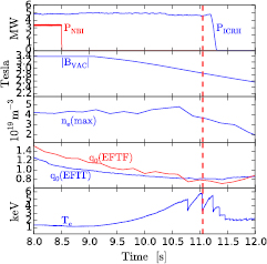
Figure 1. NBI and ICRH power, magnetic field, maximum electron density measured by LIDR Thomson scattering, safety factor on axis calculated by EFIT and EFTF and electron temperature measured by ECE through chord 72 in the late phase of discharge #92416. The vertical dashed red line indicates the time at which the antenna measurement took place.
Download figure:
Standard image High-resolution imageIn this discharge, the NBI (3.4 MW) was turned off at t = 8.5 s, which corresponds to two and a half seconds before the antenna measurement took place. This means the neutral beam injected ion population has already thermalized at t = 11.055 s, when the measurement took place. On the other hand, the ICRH (4.8 MW) was kept on until after t = 11.055 s. Both EFIT and EFTF indicate that the safety factor on axis has already dropped below unity at the time at which the measurement was performed. This is confirmed by measurements of the electron temperature carried out with ECE which show the plasma sawtoothing after t = 10.8 s. Regarding the TAE frequencies, the TAE gap is centred at the frequency f = vA/4πqR [15], where R is the major radius, vA = B/ is the Alfvén velocity, µ0 is the magnetic permeability and
  is the mass density. Throughout the current flat-top phase of the discharge, the magnetic field was B = 3.4 T and electron density was around ne = 4.3 × 10¹⁹ m−3, to which corresponds an Alfvén velocity on axis of around vA = 8 × 10⁶ ms−1. During this phase, the safety factor was dropping and, as consequence, the frequency of the TAE gap was increasing. A safety factor on axis of q0 = 1 was reached at a time around t = 10.0 s and for this value of q0 the TAE gap on axis is centred at around f = 214 kHz. Towards the end of the discharge, both the magnetic field and the plasma density decrease. At t = 12.0 s, the Alfvén velocity increased to vA = 8.97 × 10⁶ ms−1 as the decrease in density was much steeper than the decrease in magnetic field. Since at this late phase of the discharge the safety factor on axis has stabilized, the frequency of the TAE gap increases slowly due to the increase in vA. In order to cover the range of frequencies of the TAE throughout the discharge, the antenna was set to scan frequencies from f = 125 kHz to f = 250 kHz. The zig-zag line in figure 2 indicates the temporal evolution of the antenna frequency.
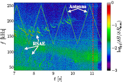
Figure 2. Magnetic spectrogram from Mirnov coils of the late phase of discharge #92416. The vertical dashed red line indicates the time at which antenna measurement took place.
Download figure:
Standard image High-resolution imageMore information on this discharge can be obtained by looking at the magnetic spectrogram (see figure 2).
Alfvén cascades (AC) [16], also known as reversed shear Alfvén eigenmodes (RSAE), are clearly visible up to t = 9.5 s and seem to last, though less clearly, up to t = 10.2 s, indicating the q-profile is reversed during this period. As the discharge progresses, the safety factor on axis gradually drops. First sawtooth crash is observed at around t = 10.8 s, indicating that at this time the safety factor on axis has already dropped below unity, which is in agreement with both EFIT and EFTF. As the safety factor on axis drops, the q-profile eventually becomes monotonic. Both EFIT and EFTF indicate a monotonic q-profile at the time at which the antenna measurement took place (t = 11.055 s). Finally, it is worth to note that after around t = 10.2 s, all Alfvénic activity is supressed, with exception of a few short lived and very low amplitude modes at around t = 10.7 s. Interestingly, half of the modes observed around t = 10.0 s have negative toroidal mode numbers i.e. propagate opposite to the plasma current. The stabilization of the Alfvénic activity suggests the drive provided by the ICRH accelerated population was decreasing. At the time at which the antenna measurement took place, all Alfvénic modes were stable.
3. Alfvén eigenmode active diagnostic (AEAD)
JET Alfvén eigenmode active diagnostic (AEAD) [17, 18] is composed by two groups of four antennas each, both localized below the outboard midplane at opposite toroidal locations. Each AEAD antenna consists of a rectangular coil with 18 turns of inconel wire and are separated toroidally by 5°. In the last campaign the system went in operation and through an upgrade, it was the first time that more than four antennas have been powered simultaneously due to new amplifiers available. The frequency range of 125 kHz–250 kHz was covered by the experiments. The relative phasing of the individual driving amplifiers was chosen to maximize the excitation of toroidal mode numbers |n| = 4 and |n| = 6, though the amplitude of other low |n| is still significant. The toroidal mode number of the mode being probed was not determined due to a reduced number of available magnetic probes during the experiment, which did not allow a precise n identification.
The antenna is used to excite/probe marginally stable modes and measures their damping rates as resonances in the magnetic probe signals as the antenna frequency is scanned across the resonant frequency. The measurement of the damping rate is based on the quality factor of the resonance, its width in frequency. The real and imaginary parts and complex plane representation of the signal measured in discharge #92416 at t = 11.055 s are shown in figure 3. A transfer function [19] has been fitted to obtain a normalized damping rate of γ/ω = −2.74 ± 0.59%. A negative value of γ/ω indicates the mode is being damped while a positive value indicates the mode is growing in amplitude. The points shown in figure 3 were collected during the interval [11.0 s, 11.1 s], which includes points collected during the sawtooth crash at t = 11.048 s. However, there appear to be steady-state conditions and the signal appears to be unaffected by the crash. Indeed, most of points collected during the crash are clustered, i.e. there is no change in signal.
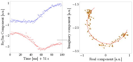
Figure 3. Real and imaginary parts (left) and complex plane representation (right) of a magnetic probe signal in discharge #92416, including points collected during the interval (11.0 s, 11.1 s). A transfer function [19] has been fitted to this data as shown.
Download figure:
Standard image High-resolution image4. Calculation of eigenmodes
Since the identification of the toroidal mode number of the mode probed by the antenna was not possible, TAEs from n = 3 to n = 6, were considered as candidates. These are the toroidal mode numbers of the modes normally probed by the antenna. The first step in the workflow leading to the calculation of the structure of these modes is the reconstruction of the equilibrium. In JET, the equilibrium can be reconstructed by the codes EFIT, EFTF or EFTM [7]. These codes are similar, except they may use different sources of data. EFIT (Equilibrium FITting) is a numerical code that performs equilibrium reconstruction based on external diagnostics like external probes and magnetic coils. Since recent times, a high temporal resolution EFIT is available at JET. EFTF is similar to EFIT but it also takes into account Faraday rotation measurements. It is not known a priori which code produces a more accurate reconstructed equilibrium. In some cases, it is possible to perform consistency checks with the observed MHD, but at the time at which the antenna measurements took place no unstable MHD modes existed. EFTM is similar to EFIT but it also uses internal data from motional Stark effect (MSE) diagnostic and it is usually seen as reconstructing the most reliable equilibria. However, at t = 11.055 s MSE was not operating as the NBI had been already turned off. Since it is not known which code yields a better equilibrium, at this stage both EFIT and EFTF were used in parallel. Due to the relatively low temporal resolution of EFTF the closest existing equilibrium was calculated for t = 11.000 s, this is, before the sawtooth crash at t = 11.048 s. On the other hand, the equilibrium reconstructed by EFIT was obtained for t = 11.097 s, this is, after the crash. Nevertheless, equilibrium reconstruction based on external diagnostics is not that much affected by core events like sawtooth crashes. The safety factor profiles reconstructed by both EFIT and EFTF are presented in figure 4.

Figure 4. Safety factor profiles reconstructed by EFIT at t = 11.097 s (solid red line), and reconstructed by EFTF at t = 11.000 s (dotted blue line). s is the square root of the normalized poloidal flux.
Download figure:
Standard image High-resolution imageThe second step of this workflow is the refinement of the equilibria reconstructed either by EFIT or EFTF. The equilibrium refinement was performed using the equilibrium code HELENA [8]. Finally, the TAE radial structure are calculated by the ideal MHD MISHKA code [9]. Being an ideal MHD code, MISHKA presents computational advantages but on the other hand it does not include resistivity, parallel electric fields or finite Larmor radius effects, which, if included, could alter both the mode structure and frequency.
Aside from the equilibrium, which is provided by HELENA, MISHKA also requires as input the mass density profile, on which the Alfvén frequency profile depends. The shape of the mass density profile was assumed to be similar to that of the electron density profile. Modes were calculated using density profiles from two distinct Thomson scattering diagnostics, the high resolution Thomson scattering (HRTS) [20] and the LIDAR Thomson scattering (LIDR) [21, 22]. The occurrence of a sawtooth crash so close to the time at which the antenna measurement took place may cause difficulties on the choice of the most adequate data to use in the simulations. However, a series of electron density profiles obtained with HRTS for time slices just before and after the occurrence of the sawtooth crash show that the effect of the crash on the profiles is not much significant. The maximum central density measured before the crash was close to ne = 3.9 × 10¹⁹ m−3. The values of the central density obtained by fitting the data were ne = 3.50 × 10¹⁹ m−3 for the profiles from HRTS, ne = 3.68 × 10¹⁹ m−3 for the profile obtained with data from LIDR/EFIT and ne = 3.74 × 10¹⁹ m−3 for the profile obtained with data from LIDR/EFTF. The last two values are slightly different because raw data from LIDR has a small peak in the centre and the mapping from R to s (square root of the normalized poloidal flux) is not coincident in EFIT and EFTF. The density profiles obtained with different combinations of data are shown in figure 5.

Figure 5. Electron density profiles fitted from LIDR/EFIT (solid red line), LIDR/EFIT (solid blue line). HRTS/EFIT (dotted red line) and HRTS/EFTF (dotted blue line). s is the square root of the normalized poloidal flux.
Download figure:
Standard image High-resolution imageFigure 6 shows the radial structures of all the n = 3 to n = 6 modes calculated with MISHKA using the density profile from LIDR and the equilibrium reconstructed by EFIT.

Figure 6. Radial structure of the n = 3 to n = 6 TAE calculated with MISHKA using data from LIDR and the equilibrium reconstructed by EFIT. Top left: n = 3, top right: n = 4, bottom left: n = 5, bottom right: n = 6.
Download figure:
Standard image High-resolution imageThe modes found with the MISHKA code are composed by two dominant poloidal harmonics and are localized in the plasma core. Such modes are classified as core-localized TAEs [23, 24]. These modes, when localized inside the q = 1 surface, are known as tornado modes and have been extensively studied in JET [25, 26]. In discharge #92416 at t = 11.055 s, ECE measurements found the sawtooth inversion radius localized at around s = 0.40, which is in fair agreement with the location of the q = 1 surface found by both EFIT and EFTF. Here, s is the square root of the normalized poloidal flux. So, all the modes found can be classified as tornado modes. It is also apparent from figure 6 that with increasing toroidal mode number, the calculated modes are located radially further outside and higher m poloidal harmonics increase in amplitude. However, the mode does not lose its core-localized nature. The n = 5 mode calculated with different combinations of data (EFIT/EFTF) and (HRTS/LIDR) are shown in figure 7. The radial structure of the n = 5 mode is nearly identical when calculated using a density radial profile obtained either from HRTS or from LIDR. This result is not surprising as the density profiles obtained with both diagnostics are very similar except in the very centre of the plasma, where the electron density measured by HRTS is somewhat lower. This does not affect the radial structure of the calculated modes though it affects the Alfvén frequency in the centre of the plasma. The modes calculated with the equilibrium reconstructed by EFTF are radially localized slightly to the outside than those calculated with the equilibrium reconstructed by EFIT. As consequence, the higher m poloidal harmonics also have higher amplitudes though the modes still keep their core-localized nature. The reason for this discrepancy in radial location stems from the transposition of the radial profiles measured in radius R to the square root of the normalized poloidal flux s as radial coordinate. Indeed, for the same radius R over the outboard midplane, EFTF associates a higher value of s than EFIT.
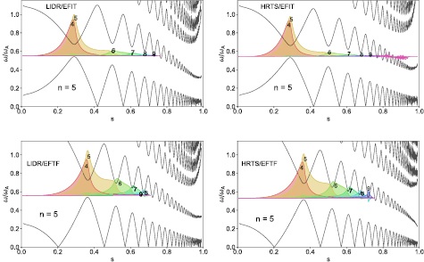
Figure 7. Radial structure of the n = 5 mode calculated with MISHKA using different combinations of data. Top left: LIDR/EFIT, top right: HRTS/EFIT, bottom left: LIDR/EFTF, bottom right: HRTS/EFTF.
Download figure:
Standard image High-resolution imageThe frequencies of the modes calculated with the MISHKA code using the different combinations of data are presented in table 1. These values compare with the antenna frequency at the time of the measurement, f = 218.3 ± 0.8 kHz.
Table 1. Frequencies of the modes calculated with MISHKA using different combinations of data.
| LIDR/EFIT | HRTS/EFIT | LIDR/EFTF | HRTS/EFTF | |
|---|---|---|---|---|
| n = 3 | f = 227 kHz | f = 232 kHz | f = 232 kHz | f = 225 kHz |
| n = 4 | f = 217 kHz | f = 219 kHz | f = 218 kHz | f = 214 kHz |
| n = 5 | f = 212 kHz | f = 214 kHz | f = 213 kHz | f = 209 kHz |
| n = 6 | f = 210 kHz | f = 210 kHz | f = 211 kHz | f = 208 kHz |
The frequencies of the modes measured experimentally are affected by a Doppler shift due to plasma rotation. The Doppler shift depends linearly on the toroidal mode number and on the plasma rotation. Since the NBI was already turned off, there are no measurements of the plasma rotation at this time (t = 11.055 s). However, since the main mechanism inducing plasma rotation in JET (and in other tokamaks as well) is the tangential injection of beam ions, this means the plasma rotation at t = 11.055 s should be small. Without NBI, the plasma rotation in JET experiments is typically around 1 kHz in the core of the plasma. This is, for example, the frequency at which n = 1 kink modes are commonly observed in experiments without NBI. Assuming the plasma is rotating with frot = 1 kHz at the location of the modes, the shift in frequency of each mode due to the Doppler effect is then equal to its toroidal mode number (Δf = n · frot). Adding this frequency shift to the values of the mode frequencies calculated with MISHKA and presented in table 1, the frequencies obtained for the n = 5 mode nearly coincide with the frequency of the antenna. The frequencies obtained for the n = 4 and n = 6 modes are also very close. For the n = 3 mode, the discrepancy between the calculated and the antenna frequencies is larger, but the difference is still relatively small, below 8%. Based on this, the mode probed by the antenna and for which the damping was measured is more likely to be an n = 4, n = 5 or n = 6, though the possibility of being an n = 3 should not be excluded.
5. Damping assessment
There are several damping mechanisms which may possibly affect the stability of the TAEs existing in the plasma, including the electron and ion Landau damping, the collisional damping, the continuum damping and the radiative damping. On the other hand, the only possible source of drive is provided by the population of energetic ions accelerated by ICRH. This population is responsible for the destabilization of several modes early on in the discharge up to around t = 10.2 s, but the drive provided by the ICRH accelerated ion population has decreased since then. As it will be shown, at the time at which the antenna measurement was performed, t = 11.055 s, the ICRH accelerated ion population is not driving the modes calculated in section 4 but it is actually damping them. Thus, all the considered modes are necessarily stable at this time as there are no driving sources. Since antenna measurements can only be performed on stable (damped) modes, these conditions are ideal for performing the measurements.
In this section, each of the terms contributing to the mode growth rate γ/ω are calculated separately. The collisional, continuum and radiative damping are assessed using the resistive MHD stability code CASTOR [10]. The contribution from the ICRH accelerated population to the mode growth rate and the electron and ion Landau damping are calculated using the CASTOR-K code [11, 12]. CASTOR-K is a drift-kinetic code which calculates the resonant exchange of energy between populations of energetic or thermal particles and MHD modes, allowing this way to assess the drive/damping of the mode associated with this transfer of energy. Since, as mentioned, it is not known which mode was probed by the AEAD antenna, the calculations of drive/damping were performed for all the modes under consideration, n = 3 to n = 6, using by default the equilibrium reconstructed by EFIT and radial profiles from LIDR. In some cases, results using different sources of data (EFTF or HRTS) are also presented in order to evaluate how the results can be affected by the choice of the sources of data.
5.1. Collisional damping
The damping of TAEs may be enhanced due to collisions of trapped electrons with passing electrons and trapped electrons with ions [27], a mechanism that is usually known as collisional damping. This damping is habitually small and may become of relevance only for modes with high poloidal harmonics m. The collisional damping can be calculated using the CASTOR code taking the value of the resistivity at the radial position of the modes. CASTOR takes as input the normalized resistivity η = ρ/(µ0R0vA(0)), where ρ is the plasma resistivity, R0 is the major radius of the magnetic axis, vA(0) is the Alfvén velocity at the magnetic axis, and µ0 is the permeability of free space. To obtain the plasma resistivity the Spitzer formula was used, ρ ≈ 2.8 × 10⁻⁸/ (with Te in keV) [28], which leads to values of the normalized resistivity between η ≈ 5 × 10⁻⁹ and 10−8, depending on the modes. The values of the collisional damping obtained with CASTOR are presented in table 2 for each of the modes considered. As it is apparent, the collisional damping is very small for all the modes under consideration.
Table 2. Collisional damping calculated with CASTOR using the equilibrium reconstructed by EFIT and radial profiles of ne and Te from LIDR.
| n = 3 → (γ/ω)coll = −2.46 × 10⁻⁴% |
| n = 4 → (γ/ω)coll = −1.03 × 10⁻³% |
| n = 5 → (γ/ω)coll = −1.96 × 10⁻³% |
| n = 6 → (γ/ω)coll = −5.35 × 10⁻³% |
5.2. Continuum damping
In ideal MHD, shear Alfvén eigenmodes may experience damping due to resonant interaction with the shear Alfvén continuum. This resonant power absorption occurs at the location where the frequency of the mode is the same as the frequency of a continuum branch. Effects such as charge separation and mode conversion occur at these resonances, resulting in damping known as continuum damping. A standard approach to calculate this damping numerically consists in representing these processes using a resistive magnetohdrodynamic (MHD) model. In these models, the continuum damping represents the limit of resistive damping as the resistivity vanishes [29]. The values of the continuum damping (γ/ω)cont were estimated with the CASTOR code using this method. These values were found to be negligible for all the modes under consideration. This is not unexpected as all the modes have very small amplitudes at the location of the intersection with the Alfvén continuum. The continuum damping was also estimated using the eigenfunctions of the equilibrium reconstructed by EFTF instead of EFIT. These eigenfunctions are somewhat displaced to outer radial locations and could possibly lead to higher values of continuum damping. However, the values of the continuum damping obtained for the eigenfunctions of the equilibrium reconstructed by EFTF are also negligible.
5.3. Radiative damping
When adding non ideal effects like parallel electric field and first order finite Larmor radius terms to the ideal MHD model, the plasma perturbations are no longer Alfvén eigenmodes following the dispersion relation ω2 =  but become kinetic Alfvén waves (KAW) with a local dispersion relation ω2 =
  (1 + ζ
 ). Here, ρi is the ion gyroradius, ζ ≡ ¾ + (Te/Ti)[1 − iδ(νe)] is a complex number and 0 < δ(νe)
  1 is a wave dissipation rate that depends on the electron collision frequency νe and arises from the parallel resistivity model due to collisions between trapped electrons and passing particles [30]. The contribution from finite energetic particles gyroradius to the local dispersion relation [31] has been neglected in the local dispersion relation. Contrary to AEs, KAWs can propagate also transverse to the magnetic field. The fraction of the mode energy stored in parallel electric-field perturbation travels along the radial direction, thus leaving the resonant magnetic surface and being eventually transferred to the trapped-electron population by Landau damping. This damping mechanism is known as radiative damping of TAEs [30, 32]. The method followed to estimate the radiative damping [30] relies on the formal equivalence between a non-ideal MHD model that accounts for finite parallel electric field and first-order ion-gyroradius effects, and the resistive MHD model that is implemented in the CASTOR eigenvalue code. Thus, the non-ideal effects can be simulated by introducing a complex resistivity in CASTOR. Since of the two components of non-ideal eigenmodes, KAWs suffer much stronger collisional damping than AEs, it is possible to infer the radiative damping by conducting a scan in δ(νe). The scan is conducted by fixing the imaginary part of the complex resistivity Im(η) [33] while the real part Re(η) and thus the equivalent value δ(νe) is increased. When the computed damping rate Im(ω)/Re(ω) becomes independent of the wave dissipation rate δ(νe), all the energy transported by the perturbed parallel electric field is transferred to the trapped electron population. At this point, the rate at which the energy is being lost matches the rate at which the energy is transported away by the perturbed parallel electric field, so the radiative damping can be approximated by (γ/ω)rad ≈ Im(ω)/Re(ω). A more detailed explanation of this method is presented in [34, 35].
Figure 8 shows the results of the δ(νe) scans performed with CASTOR. The values of the radiative damping obtained by linear fit analysis for each of the modes under consideration are summarized in table 3.
Table 3. Radiative damping calculated with CASTOR using the equilibrium reconstructed by EFIT and radial profiles of ne and Te from LIDR.
| n = 3 → (γ/ω)rad = −0.123% |
| n = 4 → (γ/ω)rad = −1.91% |
| n = 5 → (γ/ω)rad = −2.71% |
| n = 6 → (γ/ω)rad = −2.87% |
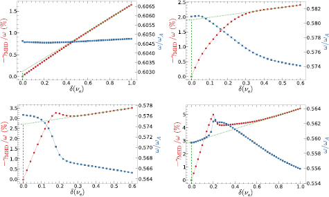
Figure 8. Estimation of the radiative damping rates for the n = 3 (top left), n = 4 (top right), n = 5 (bottom left) and n = 6 (bottom right) TAEs. Red curves represent the MHD damping rate calculated by CASTOR as a function of the wave dissipation rate whereas blue curves represent the frequency of the non-ideal eigenmode.
Download figure:
Standard image High-resolution imageThese results indicate the radiative damping is the dominant damping mechanism, except in the case of the n = 3 mode which seems not to be much affected by radiative damping. The non-ideal effects responsible for the radiative damping can be quantified through a non-ideal parameter [36] from which becomes clear that the location of the mode is a determinant factor. An analytical estimation of the radiative damping (equation (27) of [37]) shows a squared dependence on the magnetic shear S ≡ rq'/q, where q' is the radial derivative of q. The n = 3 TAE is localized closer from the core (peaks around s = 0.1) in a region of very low magnetic shear, S = 0.012 while the n = 5 and n = 6 TAE are localized around the magnetic surface s = 0.3, where S = 0.202. This suggests the n = 3 TAE experiences such a low radiative damping due to being localized in a region of very low magnetic shear.
5.4. Ion and electron Landau damping
Ion Landau damping [38] resulting from resonant interaction between bulk ions and TAE is one of the main damping mechanisms of TAE in tokamaks. Only a negligible number of bulk ions are able to interact with the TAE through the resonance v= = vA, as their parallel velocity v= is too low. However, the magnetic field curvature modifies the resonance condition reducing the parallel velocities required for achieving resonance [39] and the bulk ions can then interact with the TAE through side-band resonances, v= = vA/(2n + 1), where n is an integer. The efficiency of the interaction decreases with n, so, only low n side-band resonances effectively contribute to the damping. Electron Landau damping is a similar process involving electrons instead of ions but typically leads to lower values of damping.
The damping resulting from the resonant interaction between each of the thermal species, which in this case are electrons and deuterium ions, and each of the Alfvén eigenmodes under consideration was calculated using the CASTOR-K code. In the case of electrons, the density and electron temperature profiles used in this simulation were obtained by fitting the data measured by LIDR. Just before the antenna measurement has taken place at t = 11.055 s, a sawtooth crash has occurred at t = 11.048 s, with measurements from the fast temporal resolution ECE indicating a drop in the electron temperature in the centre of the plasma from around Te = 6 keV to Te = 3.5 keV. The value of the electron temperature in the centre of the plasma obtained from fitting LIDR data and used as input in CASTOR-K was Te = 4.2 keV, consistent with a swift partial recovery of the electron temperature after the crash. The distribution of thermal electrons in the normalized magnetic moment Λ ≡ µB0/E, where µ is the magnetic moment, was assumed to be isotropic. Since for the population of thermal deuterium ions no measurements of the radial density and temperature profiles are available, the profiles were assumed to be similar to those of the electrons. The distribution in Λ was assumed to be isotropic as well. In order to evaluate how the calculated damping depends on the choice of the sources of data, the calculation of the damping on thermal deuterium ions was also performed using the equilibrium reconstructed by EFTF and the profiles measured by HRTS instead of EFIT/LIDR.
The radial profiles of the electron temperatures obtained with LIDR/EFIT and HRTS/EFTF are shown in figure 9. The profile from HRTS has been obtained at a time slice closer from the sawtooth crash, showing a lower temperature in the centre and a flatter profile. The values of the Landau damping calculated with CASTOR-K are presented in table 4.
Table 4. Electron and ion Landau damping calculated with CASTOR-K.
| MODE NUMB. | DATA | SPECIES | DAMPING |
|---|---|---|---|
| n = 3 | LIDR/EFIT | Ion (D) | γ/ω = −0.3822% |
| n = 3 | HRTS/EFTF | Ion (D) | γ/ω = −0.0311% |
| n = 3 | LIDR/EFIT | Electron | γ/ω = −0.0324% |
| n = 4 | LIDR/EFIT | Ion (D) | γ/ω = −0.0507% |
| n = 4 | HRTS/EFTF | Ion (D) | γ/ω = −0.0324% |
| n = 4 | LIDR/EFIT | Electron | γ/ω = −0.0216% |
| n = 5 | LIDR/EFIT | Ion (D) | γ/ω = −0.0517% |
| n = 5 | HRTS/EFTF | Ion (D) | γ/ω = −0.0334% |
| n = 5 | LIDR/EFIT | Electron | γ/ω = −0.0228% |
| n = 6 | LIDR/EFIT | Ion (D) | γ/ω = −0.0564% |
| n = 6 | HRTS/EFTF | Ion (D) | γ/ω = −0.0329% |
| n = 6 | LIDR/EFIT | Electron | γ/ω = −0.0262% |
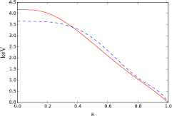
Figure 9. Electron temperature profiles fitted from LIDR/EFIT (solid red line), and HRTS/EFTF (dotted blue line).
Download figure:
Standard image High-resolution imageThe numerical results show the Landau damping is quite small in all cases except in the case of the n = 3 mode solution of the equilibrium reconstructed by EFIT. This is due to the fact that this mode is localized radially further inside than all others (see figures 6 and 7). In this region, the density and temperature of the plasma are higher leading to a larger Landau damping. In general, the values of the ion Landau damping calculated for the modes obtained using the equilibrium reconstructed by EFIT are higher than those calculated for the modes obtained using the equilibrium reconstructed by EFTF. This is also due to the localization of the modes, which in the first case are closer from the plasma centre. The simulations also show that low n TAEs are damped by strongly passing and passing ions (low Λ) and as the toroidal mode number increases, the damping contribution from trapped ions also increases. Concerning the damping of the TAEs on electrons, it is due to resonant interaction with trapped electrons as only these electrons are in resonance with the modes.
5.5. Contribution to γ/ω from the ICRH minority population
At t = 11.055 s, 4.8 MW of ICRH are still being applied on the plasma, so it still contains a significant population of energetic hydrogen minority ions. These ions potentially drive TAEs via resonant interaction. Their contribution to the mode growth rates has been calculated using the CASTOR-K code. In this code, the distribution function of the energetic ion population is given as function of the radial density (from which the toroidal canonical momentum Pφ is obtained), the energy E and the normalized magnetic moment Λ. Normally, the ICRH is applied on-axis, which was the case of discharge #92416 during the current flat-top phase. For on-axis heating, the ICRH accelerated population distribution is peaked near the plasma centre and the ions efficiently accelerated by ICRH are those moving in banana orbits whose tips fall over the ICRH resonant layer. A common approximation is to assume the whole energetic ion population to be characterized by a single Λ, which is given by the ratio between the major radius of the resonant layer and the magnetic radius Λ = Rres/R0. Thus, for on-axis heating, the whole energetic ion population is characterized by Λ = 1.
In the case under analysis, the AEAD antenna measurement was performed late on the discharge and at the time at which the measurement was performed (t = 11.055 s), the magnetic field was already ramping down (see figure 1), implying the ICRH resonance layer was moving inward in major radius. The change in the location of the ICRH resonance layer has important implications on the stability of the TAE. Most importantly, it changes the radial location of the peak in density of the energetic ion distribution, which is crucial for TAE stability as the TAE are excited through radial gradients of the energetic ion distribution. Aside from it, it changes the type of orbits of the accelerated ions, which become barely trapped ions when the ICRH resonance layer moves inward in major radius, and changes the distribution in energy of the energetic ion population.
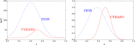
At t = 11.055 s, the ICRH resonance layer was localized at Rres = 2.559 m which, over the midplane, corresponds to s = 0.517 and Rres/R0 = 0.865. The radial distributions of the energetic ion density and temperature have been calculated both with the PION code [40] and with the CYRANO/StixRedist codes. CYRANO [41] is a 2D full-wave code that calculates the absorption of the radio-frequency waves throughout the plasma. The StixRedist code [42] takes the output of CYRANO as input and solves the Fokker–Plank equation to calculate the density and energy distribution of the ICRH accelerated population by using the Stix model [43]. CYRANO/StixRedist found a radial distribution of energetic ions steeply peaked and centred near the magnetic flux surface that is crossed by the ICRH resonant layer over the midplane. This code predicts the energetic ion temperature to peak around the same location as the density, reaching a maximum temperature of THOT = 50 keV at the peak. On the other hand, PION predicts the energetic ion density profile to be less steeped and peaked closer from the core, at around s = 0.35. The energetic ion temperature predicted by PION goes up to THOT = 190 keV on its peak. The differences in the peak tail temperatures and their radial localizations as calculated by CYRANO and PION are mainly due to the differences in the modelling of the ICRH-driven fast ion distribution function in the two codes. The wave-solver CYRANO is coupled with a 1D Fokker–Planck model of the ICRH driven fast ion distribution based on the Stix formalism without taking into account finite orbit width effects. It solves the steady state fast ion distribution function at a given time point in the discharge. PION evolves the fast ion distribution and the ICRH wave power deposition self-consistently in time throughout the discharge and includes a simplified model to account for finite orbit width effects of ICRH driven fast ions. In the time interval of our interest in discharge #92416, the magnetic field was ramped down, moving the off-axis ICRH resonance further to the high-field side. In these conditions the above differences in the modelling of the fast ion distribution function resulted in a higher peak tail temperature located at a smaller minor radius in PION as compared with CYRANO. The radial profiles of energetic ion temperature and normalized density reproducing PION and CYRANO results and given as input to CASTOR-K are shown in figure 10.
Figure 10. Radial profiles of the energetic ion temperature (left) and normalized density (right) reproducing PION and CYRANO results and which were used as input in CASTOR-K. The actual density is obtained by matching the number of energetic ions used in the simulations with the number predicted to exist in the experiment.
Download figure:
Standard image High-resolution image
The effects of the resonant interaction between the ICRH accelerated ion population and the TAEs under consideration as calculated by CASTOR-K are presented in table 5. The results were obtained using the energetic ion distribution function calculated by CYRANO/StixRedist, the mass density profile obtained with data from LIDR and the equilibrium reconstructed by EFIT.
Table 5. Contribution to the TAEs growth rate resulting from the resonant interaction with the ICRH accelerated population as calculated with CASTOR-K. The energetic ion distribution was calculated by CYRANO/StixRedist, the equilibrium was reconstructed by EFIT and density profile was obtained from LIDR data.
| n = 3 → (γ/ω)ICRH = −1.61 × 10⁻⁵% |
| n = 4 → (γ/ω)ICRH = −3.0 × 10⁻³% |
| n = 5 → (γ/ω)ICRH = −0.025% |
| n = 6 → (γ/ω)ICRH = −0.09% |
Results presented in table 5 show that the off-axis ICRH accelerated population is not transferring energy to any of the TAEs, but instead it is actually damping the modes. The results from table 5 are easily understandable. The modes are being damped instead of driven because the energetic ion population peaks at an outer location than the amplitude of the modes, so the resonant interaction occurs in a region where the radial density gradient is positive. The damping is small because the energetic ion density and temperature are small at the location of the modes and the damping increases with the toroidal mode number because modes with higher n are localized closer from the peak of the energetic ion density. If the energetic ion population calculated by PION is considered instead of that from StixRedist, then the modes become localized in a region of high density of energetic ions and the damping becomes much higher, up to around (γ/ω)ICRH = −3.0% for the modes with the highest damping.
The fact that all Alfvénic activity is suppressed just after t = 10 s and afterwards the ICRH resonant layer moves further off-axis suggests the effect of the ICRH accelerated population on the TAE must be small at the time of the antenna measurement.
6. Summary and conclusions
The new AEAD JET antennas system has been used to measure the damping of TAE modes in discharge #92416. The system does not allow a direct control over which modes the antenna probes, so frequencies in the range from 125 kHz to 250 kHz were scanned and the relative phasing between individual driving amplifiers was chosen to maximize the excitation of |n| = 4 and |n| = 6 modes. If the antenna resonates strongly enough with a damped mode, then the mode can be probed. A damping measurement was performed at t = 11.055 s and this value was compared with the results from numerical calculations which include all possible relevant sources of damping/drive obtained by using different sets of numerical codes. These include the collisional damping, radiative damping, continuum damping, Landau damping on thermal species and resonant interaction with the ICRH accelerated population. Since the toroidal mode number of the TAE for which the measurement was performed could not be determined experimentally, calculations were performed for a range of modes with toroidal mode numbers between n = 3 and n = 6 and frequency matching has been used to identify which mode was possibly probed by the antenna. The agreement between the experimental frequency of the mode probed by the antenna and the frequency of the modes calculated by MISHKA is very good. The radial structure of the modes calculated with the MISHKA code indicates these modes are core-localized TAE inside the q = 1 surface (tornado modes). Since the dominant poloidal harmonics of these modes are vanishing towards the plasma edge, the coupling must be established via higher order sidebands, a mechanism which has still to be understood.
The damping calculations show that the radiative damping is largely dominant over all other sources of damping except for the n = 3 TAE, for which the radiative damping is small. The off-axis ICRH accelerated population was found to be also damping the TAE under consideration instead of driving. Continuum damping, collisional damping and ion and electron Landau damping were found to be very small, except the ion Landau for the n = 3 TAE, as this mode is localized close to the centre in a region where the thermal density and temperature are higher. Table 6 shows the overall damping obtained for each mode, taking into account all considered sources of damping.
Table 6. Overall damping rate for each mode taking into account all considered sources of damping. Data used is from EFIT/LIDR and the energetic ion distribution function is from CYRANO.
| n = 3 → γ/ω = −0.50% |
| n = 4 → γ/ω = −1.96% |
| n = 5 → γ/ω = −2.79% |
| n = 6 → γ/ω = −3.01% |
The damping rate measured by the antenna is γ/ω = −2.74 ± 0.59%. The agreement in frequency and calculated damping is very good for the n = 5 and n = 6 TAEs, one of these being probably the mode probed by the antenna. The measured damping is basically radiative damping.
Acknowledgments
This work has been carried out within the framework of the EUROfusion Consortium and has received funding from the Euratom research and training programme 2014-2018 under grant agreement No 633053. IST activities also received financial support from 'Fundação para a Ciência e Tecnologia' through project UID/FIS/50010/2013. The views and opinions expressed herein do not necessarily reflect those of the European Commission. Support for the US group was provided by the US DOE under Grant Number DE-FG02-99ER54563.