
Abstract
We discuss the origin of uncertainties in the results of numerical simulations of low-temperature plasma sources, focusing on capacitively coupled plasmas. These sources can be operated in various gases/gas mixtures, over a wide domain of excitation frequency, voltage, and gas pressure. At low pressures, the non-equilibrium character of the charged particle transport prevails and particle-based simulations become the primary tools for their numerical description. The particle-in-cell method, complemented with Monte Carlo type description of collision processes, is a well-established approach for this purpose. Codes based on this technique have been developed by several authors/groups, and have been benchmarked with each other in some cases. Such benchmarking demonstrates the correctness of the codes, but the underlying physical model remains unvalidated. This is a key point, as this model should ideally account for all important plasma chemical reactions as well as for the plasma-surface interaction via including specific surface reaction coefficients (electron yields, sticking coefficients, etc). In order to test the models rigorously, comparison with experimental 'benchmark data' is necessary. Examples will be given regarding the studies of electron power absorption modes in O2, and CF4–Ar discharges, as well as on the effect of modifications of the parameters of certain elementary processes on the computed discharge characteristics in O2 capacitively coupled plasmas.
Export citation and abstract BibTeX RIS

Original content from this work may be used under the terms of the Creative Commons Attribution 3.0 licence. Any further distribution of this work must maintain attribution to the author(s) and the title of the work, journal citation and DOI.
1. Introduction
The number of numerical modelling/simulation studies of low-temperature plasma sources has been rapidly growing during the last two decades, thanks to the fast advance of computational tools. This trend is expected to continue due to the high interest in applications of low-temperature plasmas [1, 2] in various branches of the high-tech industry. Besides 'homebrew' codes, simulation software available as freeware, as well as commercial tools, are also at the disposal of modellers.
The reliability of the computational results depends on (i) the validity of the physical model of the given system and (ii) the correctness of the implementation of the model in the simulation code. The latter is examined in the verification process [3], in which the code or parts of the code are executed for problems for which analytical solutions are known. In the absence of this possibility, comparison of the results of independent codes implementing the same model—known as benchmarking—can provide evidence for the correctness of the implementations. Such a study, for five independent radio-frequency discharge plasma simulation codes, has been presented in [4]. The correctness of a model itself can be addressed in the validation process, when the simulation results are cross-checked with experimental data, e.g., [5–8]. To reach reliable conclusions it is necessary to measure a number of different physical quantities in the experiment over a wide range of operating conditions. Careful parametric investigations of plasma sources equipped with a variety of diagnostics tools can provide experimental benchmark data for this purpose. As an example of such a recent study, we quote measurements on low-pressure capacitively-coupled radio-frequency oxygen plasmas [9, 10] that were driven by single- and multi-frequency (peaks- and valleys-type) voltage waveforms [11, 12] with different peak-to-peak voltage amplitudes over a wide range of pressures. These experiments provided the dc self-bias voltage (in the case of multi-frequency waveforms), the ion flux and the flux-energy distribution of (mass-selected) positive ions at the grounded electrode, the power absorbed by the discharge and spatio-temporal maps of electron power deposition as obtained from phase-resolved optical emission spectroscopy (PROES) [13]. In [9, 10], these experimental results have been rigorously compared to results of particle-in-cell/Monte Carlo collision (PIC/MCC) simulations [14] using our own code.
In general, a model and the simulation tool based on it, can be considered as a box that has a certain number of inputs and a certain number of outputs (see figure 1). Part of the inputs defines the operating conditions (voltage amplitude and waveform, gas pressure and composition, electrode separation, etc) and the other part consists of the physical input data of rate coefficients, cross-sections, transport coefficients, coefficients characterising surface processes, etc. The output quantities are the discharge characteristics: the particle densities, fluxes, and energy distributions, electric field distribution, etc. The input and output quantities can both be scalars (e.g., ion flux at an electrode) or functions (e.g., energy dependent cross-sections or ion flux-energy distributions). The output functions can depend on one or more variables: e.g., the total current flowing in a radio-frequency discharge is a function of time only, but the electron conduction current is a function of time and space. For some input quantities, there is a choice between handling them as scalars (simple approach) or as functions (more refined approach); e.g., the secondary electron emission coefficient is often approximated as a constant value, whereas other studies consider its dependence on particle energies and surface conditions [15–19].

Figure 1. A description of the modelling process.
Download figure:
Standard image High-resolution imageThe input and output quantities are connected 'within the box' in a complex manner via charged particle transport and plasma-chemical collision processes. The data that govern these processes—rate coefficients, cross-sections, transport coefficients, etc—originate either from theoretical calculations and/or from dedicated experiments. In both cases, these data have some uncertainties. While this is (or, actually should be) a question of paramount interest, it is very rarely asked how the accuracy of the input data affects the output data (i.e. the simulation results). As a first approximation to the answer, we can agree with the statement in the title of a work by Bogaerts and Gijbels: 'Modelling network for argon glow discharges: the output cannot be better than the input' [20]. In a more sophisticated approach of sensitivity analysis [3] one may ask the question to what degree an output quantity Oj is influenced by an input quantity Ik. One expects to find sensitivities of varying degree when scanning over all j-s and k-s. Such a complete scan is of course an immense task and, therefore, it is rarely considered.
Besides the uncertainties of the input data the assumptions of the model itself have a consequence on the accuracy of the computed quantities. While one may want to develop a model that closely reflects reality, it is also the task of modellers to find a limited set of the most important processes required to describe the system in order to keep the model (relatively) transparent. (This input to the model is represented as 'Knowledge' in figure 1.) Finding this set for a given system is aided by the possibility of switching on and off individual processes in the computations. It has also to be mentioned that the parameters of the computations themselves (time step, number of particles traced in particle-based simulations, see e.g. [21, 22]) have an effect as well on the output quantities and this sensitivity should ideally also be kept in mind.
The above thoughts lead to the conclusion that (i) the construction of discharge models is indeed a delicate task, (ii) the implementation of the model in a code has to be tested (verified, or at least benchmarked with other independent codes), (iii) the modelling results have to be handled with caution because of the various sources of uncertainties that are not well known and understood in most cases, and (iv) the models can be validated only by a thorough comparison with experimental results, preferably over a wide parameter domain. In connection to this last point we note that reliable experimental data for this purpose are generally missing, and that one should bear in mind that a thorough comparison is only possible if the geometry of the experiment can be correctly described in the simulation.
In this work, we present some examples of discharge modelling for which an acceptable agreement between simulation results and experimental benchmark data has been reached. In section 2, we focus on oxygen discharges while, in section 3, we discuss the case of CF4–Ar plasmas. Section 4 gives our conclusions.
2. Oxygen discharges
Experiments on capacitively-coupled oxygen discharges [9, 10] have been carried out at LPP (Laboratoire de Physique des Plasmas) in the DRACULA reactor [23]. This (cylindrically symmetric) reactor is equipped with aluminium electrodes with a diameter of 50 cm, separated by a distance of L = 2.5 cm. The powered electrode is connected to a class A, broad band RF power amplifier via a blocking capacitor. The control system (involving a sophisticated feedback network) allows applying arbitrary voltage waveforms to the powered electrode. The electrical characterisation of the discharge is assisted by a SOLAYL voltage–current probe and the ion flux-energy distribution function (IFEDF) is measured with a HIDEN EQP mass/energy spectrometer. Measurements of the self-bias, the power absorbed by the plasma, the flux as well as the IFEDF have been taken for single- and multi-frequency (peaks- and valleys-type) excitation waveforms for voltage amplitudes between 50 and 250 V, within the 50 and 380 mTorr pressure range. In [9], good agreement was found between the discharge characteristics obtained from these experiments and PIC/MCC simulations. PROES studies have been conducted, in a similar reactor geometry (with smaller electrode diameter of 12 cm) [10], to gain information about the electron power absorption dynamics of the plasma.
Here, we consider discharges driven by 'peaks-type' and 'valleys-type' voltage waveforms:
where N is the number of harmonics that have amplitudes and phase angles,  and
and  , respectively, f1 is the fundamental radio frequency, and

where  is the peak-to-peak voltage. The peaks-type voltage waveforms are generated by setting all phase angles to zero, while valleys-type waveforms are obtained by changing the phase angles of all the even harmonics to
  . We note that for peaks-type (valleys-type) voltage waveforms, a negative (positive) self-bias voltage develops to ensure flux compensation at the electrodes.
Our discharge model for oxygen and its (1d3v) PIC/MCC implementation has largely been based on the well-established 'xpdp1' collision cross-section set [24]. Compared to the original xpdp1 set, we replaced the elastic collision cross-section with the elastic momentum transfer cross-section of Biagi [25] (and used, accordingly, isotropic electron scattering), replaced the original xpdp1 cross-section of ionisation with that recommended by Gudmundsson et al [26], and adopted as well all the cross-sections for heavy particle processes (ion–molecule and ion–ion collisions) from [26]. In the present study, the same model for oxygen discharges is used as in [9, 10]. The electrodes are considered perfect absorbers of electrons and the emission of secondary electrons is neglected. The gas temperature is fixed at Tg =300 K. A detailed description of the model can be found in [9].
It is known that, among the surface processes in oxygen CCPs, the surface destruction probability (also called surface quenching probability) of oxygen singlet delta  molecules, α, is a very important parameter [27]. In our previous studies [9, 10], we have found that the best agreement between the experimental PROES data and simulation results for the excitation rate can be achieved for a wide domain of conditions when using a value of
  . As an illustration of the good agreement between experiment and simulation, we show in figure 2 PROES maps for the excitation rate of the O 3p3P state compared to spatio-temporal distributions of the corresponding dissociative excitation rate of the same state obtained from PIC/MCC simulations for oxygen discharges driven by valley-type waveforms, operated at f1 = 15 MHz, p = 150 mTorr,
  with different number of harmonics (N). At N = 1, both (the experimental and simulation) plots are nearly 'symmetric' (the same patterns appear at both electrodes at times shifted in time by half an RF period). The most intense excitation originates near the edges of the expanding sheaths, however, excitation also occurs in the whole bulk region, indicating that the discharge operates in a hybrid alpha—drift-ambipolar power absorption mode [29]. At N = 2, and even more at N = 3, the excitation patterns become asymmetric. For these types of excitation waveform, a faster sheath expansion is observed at the grounded electrode (situated at x = 2.5 cm in the panels of figure 2); consequently, the most intense excitation occurs near the expanding sheath edge at the top (grounded) electrode and excitation in the bulk region becomes weaker. The simulation results clearly reproduce the main features of the experimental distributions, albeit they indicate slightly less excitation/emission within the bulk. This degree of agreement, nonetheless, gives strong evidence for the overall qualitative correctness of the model.

Figure 2. PROES results ('EXP', upper row) for the spatio-temporal distribution of the electron impact excitation rate of the O 3p3P state and the distribution of the corresponding dissociative excitation rate as obtained from PIC/MCC simulations ('SIM', bottom row) in oxygen discharges driven by valley-type waveforms, operated at different number of harmonics (N). The base harmonic frequency is f1 = 15 MHz. The powered electrode is at x = 0 cm, while the grounded electrode is at the top of the panels, at x = 2.5 cm. The white lines in the bottom row mark the sheath edges determined according to [36]. Discharge conditions: p = 150 mTorr,  ,
,  . The colour scales are given in arbitrary units.
Download figure:
Standard image High-resolution imageNext, we address the question of how the changes of certain physical input parameters influence the computational results. For this study, we select only a few processes, as a complete scan over all parameters and their different combinations would be prohibitively laborious. Among the elementary processes taking place in an oxygen plasma, the cross-sections of the electron-impact processes are generally considered to be more reliable compared to those for ion–molecule reactions, for which the data in the literature are considerably scattered. Therefore, we proceed with testing the effect of the modification of the surface destruction probability, α, as well as the cross-sections of a few 'heavy-particle' processes, listed in table 1. (For the complete list of collision processes considered in our model, the reader is referred to [9].)
Table 1. List of elementary processes being analysed in the case of oxygen plasmas. For the explanation of 'Base values' and 'Base factors' see the text.
| Reaction | Process | Base value | Base factor |
|---|---|---|---|
|
Surface destruction |

|
|
|
Elastic scattering |

|
I = 0.5 |
|
Mutual neutralisation |

|
M = 1.0 |

|
Associative detachment |

|
D = 1.0 |
- The first process we study is the surface destruction of the singlet-delta oxygen molecules, α. The 'base value' for the probability of this process is set to
 . We shall test the effect of using 10 times higher and 10 times lower values in the simulations.
 - The second process that we examine is the elastic collision. In [26], this process is referred to as charge exchange and an additional process of isotropic elastic scattering with a cross-section that has 50% magnitude of the charge exchange cross-section is additionally included, i.e. , with . According to the above, the base value of the cross-section for the isotropic channel is and the base factor is I = 0.5. This factor will be changed in the following to I = 0 and to I = 1.0 to reveal the effect of this process on the computed characteristics. (Note that we follow the recommendation of Phelps [28] for the terminology, and name both charge exchange and the additional isotropic channel as elastic scattering.)
- The third process that we examine is the mutual neutralisation. We shall change the cross-section of this process (adopted from [26]) with respect to its recommended value to , using the factors M = 0.5 and 1.5.
- Likewise, we vary the cross-section of the associative detachment process (taken from [26]) with respect to the base value, to . Besides the base factor D = 1, factors of D = 0.5 and 1.5 will be used in the simulations.


The computations with these (rather drastically) modified input parameters have been carried out for discharges driven by a peaks-type voltage waveform with N = 3 harmonics, for  ,
,  = 150 V, p = 100 mTorr. The results are summarised in table 2. The first row of data gives the measured values, the second row gives the simulation results with the base values of the parameters. The additional 12 lines correspond to the parameter variations (listed above).
Table 2.
Self-bias voltage (η, in units of Volts), discharge power P (in units of Watts), and the flux of  ions at the grounded and powered electrodes,
  and
and  , respectively (in units of 1014 cm−2 s−1), as obtained in the experiment ('EXP') and in the computations with the base settings of the parameters ('BASE') and for different parameter variations (Cases 1...12). Discharge conditions: peaks-type excitation waveform with N = 3 harmonics,
  ,
,  = 150 V, p = 100 mTorr. (In the experiment only the flux at the grounded electrode was possible to measure. The flux at the powered electrode for a peak-type waveform in this case is assumed to be equal to the flux at the grounded electrode with an 'inverted' excitation waveform, i.e. using a valleys-type waveform.)
| Case | α | I | M | D | η | P |

|

|
|---|---|---|---|---|---|---|---|---|
| EXP | — | — | — | — | −36 | 7.8 | 0.63 | 0.74 |
| BASE |

|
0.5 | 1 | 1 | −39 | 12.1 | 0.57 | 0.64 |
| 1 |

|
0.5 | 0.5 | 1 | −40 | 12.6 | 0.60 | 0.67 |
| 2 |

|
0.5 | 1.5 | 1 | −39 | 11.7 | 0.53 | 0.61 |
| 3 |

|
0.5 | 1 | 0.5 | −40 | 13.9 | 0.70 | 0.73 |
| 4 |

|
0.5 | 1 | 1.5 | −39 | 10.8 | 0.48 | 0.59 |
| 5 |

|
0 | 1 | 1 | −37 | 7.4 | 0.35 | 0.49 |
| 6 |

|
0 | 1 | 1 | −40 | 13.0 | 0.65 | 0.72 |
| 7 |

|
0 | 1 | 1 | −41 | 18.1 | 1.10 | 1.00 |
| 8 |

|
0.5 | 1 | 1 | −37 | 7.1 | 0.31 | 0.45 |
| 9 |

|
0.5 | 1 | 1 | −41 | 16.8 | 0.93 | 0.88 |
| 10 |

|
1 | 1 | 1 | −37 | 6.7 | 0.29 | 0.42 |
| 11 |

|
1 | 1 | 1 | −39 | 11.5 | 0.49 | 0.58 |
| 12 |

|
1 | 1 | 1 | −41 | 15.8 | 0.81 | 0.78 |
The agreement between the experimental ('EXP') data and the simulation results with the base parameter setting ('BASE') is very good for the bias voltage and the fluxes, while the computed discharge power is ≈50% higher as compared to the experimental value. This mismatch, as shown in table 2, can be improved by changing some of the parameters, e.g. cases 5 and 10, with  give a lower absorbed power, in better agreement with the experimental value. In these cases, however, the computed
  fluxes become a factor of two lower than the experimental value (that is expected to be dominated by
  ions). The results suggest that a much better agreement cannot be reached within the degrees of freedom given by the variation of the parameters selected here. Nonetheless, these data provide information about the sensitivity of the numerical results on the parameters of the selected processes. An important outcome of this study is also a confirmation of the theoretical prediction that the self-bias voltage shows very little sensitivity to any of the parameters. In other words, η is not a good choice in any validation study. The discharge power and the ion flux represent much better choices, due to their sensitivity on process parameters.
Further results of the parameter variation are presented in the forthcoming figures. Figure 3 shows the spatial distribution of the charged particle densities as obtained in the base simulation and with modified cross-sections for mutual neutralisation (M) and associative detachment (D) processes, at fixed  and I = 0.5 (cases 1...4 in table 2). Panel (a) displays the effect of the variation of M at D = 1. The densities turn out to be relatively insensitive to the variation of the cross-section of the mutual neutralisation process; a factor of 3 change of M results in a factor 1.5 change of the peak ion densities. In the case of the associative detachment process, a similar variation of D (at fixed M = 1, see figure 3(b)) results in a change of a factor of 2 in the peak ion densities.
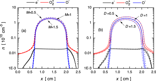
Figure 3. Computed density distributions of charged particles in oxygen plasmas; (a) effect of M at D = 1 and (b) effect of D at M = 1.  and I = 0.5 for all cases. Discharge conditions: peaks-type excitation waveforms with N = 3 harmonics, ϕ = 150 V, p = 100 mTorr.
Download figure:
Standard image High-resolution imageThe simulated charged particle distributions, for the variation of the surface destruction probability (α) and the parameter I, are shown in figure 4 at the fixed base values of the parameters M and D. Panels (a)–(c) show the density distributions at fixed I = 0.5, as a function of α. At a low,  value of the surface destruction probability, the peak densities decrease and the sheath widths increase significantly with respect to the base case (panel (b),
  ). Increasing α leads to enhanced electron densities (panel (c)). This behaviour is governed by the importance of the singlet metastable molecules in controlling the density of negative oxygen ions via the associative detachment process. (Recall that negative ions normally cannot escape the plasma bulk and, therefore, their density is set by the balance of creation and gas-phase loss processes.) The changed widths of the sheaths (as a consequence of changing α) are expected to influence the flux-energy distributions of the ions reaching the electrodes, as confirmed later on.

Figure 4. Computed density distributions of charged particles in oxygen plasmas for different combinations of the parameters α and I. D = 1 and M = 1 for all cases. The base case corresponds to  and I = 0.5 (panel (b)). (a)–(c) show the effect of varying α, while (d)–(f) show the consequences of changing the parameter I. Discharge conditions: peaks-type excitation waveforms with N = 3 harmonics,
  ,
,  = 150 V, p = 100 mTorr.
Download figure:
Standard image High-resolution imageThe magnitude of the isotropic scattering channel in the elastic  + O2 collisions has a weak influence on the charged particle densities, as revealed in figures 4(d)–(f). A higher total cross-section makes the transport of ions more collisional. Therefore, the densities slightly increase with the increase of I. This parameter, however, has a quite significant effect on the IFEDFs, shown in figure 5 for an excitation waveform with 3 harmonics, ϕ = 150 V, at 100 mTorr pressure, as the collisionality directly influences the free paths of the ions within the sheaths. Besides the influence of the parameter I on the IFEDF, the effect of varying α is also depicted in figure 5. In addition to the computed IFEDFs, those measured experimentally are also shown in selected panels of this figure, where these distributions agree reasonably well with the computed distributions. We find a satisfactory agreement in panel (e) that corresponds to the base case. The agreement can be improved by changing either α to a value of
  (panel (d)), or even more by increasing I to 1.0 (panel (h)). One should note, however, that (i) the first change results in markedly lower ion fluxes causing a higher deviation from the experimentally obtained values compared to that seen with the base values of the parameters (see table 2), whereas it improves the agreement of the computed power with the experimental value; (ii) the second choice also weakens the agreement between the computed and experimental values of the positive ions fluxes at the electrodes.
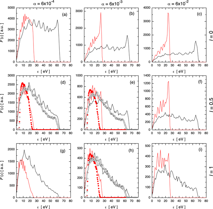
Figure 5. Flux energy distributions of the  ions at the grounded electrode, for different combinations of the parameters α and I. Black colour: peaks-type, red colour: valleys-type waveforms. The lines are simulation results while the symbols correspond to experimental data. The experimental data are shown only for the base case (panel (e)) and for cases when a good agreement between the experimental and simulation data are found (panels (d) and (h)). Discharge conditions: peaks-type excitation waveforms with N = 3 harmonics,
  , ϕ = 150 V, p = 100 mTorr.
Download figure:
Standard image High-resolution imageThis rather limited study leads us to the conclusion that refinement of the model and adjustment of the cross-sections of the individual processes is an immense task even in the case of a gas, like oxygen, for which the processes are relatively well known and have been studied for decades.
3. CF4–Ar discharges
Investigations of capacitively-coupled CF4–Ar discharges driven by different tailored excitation waveforms (including those specified in the previous section), at different pressures and gas mixing ratios, have recently been conducted at WVU (West Virginia University). These parametric studies provide a batch of experimental benchmark data which are being used now for the validation of the model of CF4–Ar plasmas. Detailed results of these ongoing investigations will be presented elsewhere. Here, we restrict ourselves to the illustration of the effect of the gas mixing ratio on the electron power absorption mode transition.
In the (homebrew) PIC/MCC code for CF4–Ar plasmas, the cross-sections of electron-CF4 collision processes are taken from [30], with the exception of the electron attachment processes (producing CF3− and  ions), for which we use data from [31]. This electron-impact collision set includes numerous processes, but the only products considered (i.e. traced in the code) are CF3+, CF3−, and F− ions, which play the most important role in CF4 discharge plasmas. For electron-Ar atom collisions, we use the cross-sections from [32] while the Ar+ + Ar cross-sections are taken from [28]. The Ar+, CF3+, CF3−, and F− ions can participate in various ion–molecule reactive processes, as well as in elastic collisions for which the cross-sections are adopted from [33]. The ion–ion recombination rate coefficients are taken from [34], while the rate for the electron-CF3+ recombination process is from [35]. In the simulations, we take the gas temperature to be 350 K, and assume that the electrons reaching the electrodes are reflected with a probability of 0.2. We have carried out simulations with
  and 0.4 values of the secondary electron emission coefficient (which are here independent of particle energies and discharge conditions). The lower value of γ is a typical choice in discharge simulations with metal electrodes, while the higher value approximates the electron yield of dielectric surface layers that may form in the experimental system over the stainless steel electrodes after a prolonged operation in CF4 gas.
In the PROES measurements, the electron-impact excitation rate from ground-state F atoms to the excited F-level responsible for the 703.7 nm emission is derived from deconvoluted space and time resolved images acquired with a nanosecond-gated, high repetition rate ICCD camera (Andor iStar) synchronised with the applied RF voltage waveform. The scenario is approximated in the simulation using the cross-section for the electronic excitation process for CF4 having a threshold of 7.54 eV by specifically accumulating excitation data for electrons with energies equal to or higher than 14.5 eV (for more details see [38]).
Figures 6(a) and (b) show experimental PROES maps, obtained as explained above, for CF4–Ar discharges at 0% and 90% Ar content, at p = 450 mTorr and  = 150 V voltage amplitude. Due to the specific design of the reactor (GEC cell), the asymmetry of the discharge was unavoidable. Nonetheless, the excitation patterns in the case of the pure CF4 discharge (figure 6(a)) clearly reveal the drift-ambipolar electron power absorption mode, where electrons primarily absorb power in the bulk plasma and at the edge of the collapsing sheath. This latter is most prominent at the edge of the collapsing sheath at the powered side of the discharge. The simulation results clearly corroborate this behaviour, as shown in figures 6(c) and (e), corresponding, respectively, to the simulations executed with the
  and
and  values of the secondary electron emission coefficient.

Figure 6. PROES maps ('EXP', panels (a) and (b)) and spatio-temporal distributions of the electron impact excitation rate obtained from PIC/MCC simulations ('SIM', panels (c), (d)) for  and panels (e), (f) for
  (secondary electron emission coefficients) for CF4–Ar discharges with 0% (left column) and 90% (right column) Ar content. The discharges are driven by a single harmonic waveform. The powered electrode is situated at x = 0, while the grounded electrode is at x = 2.5 cm.
  is the period of one RF cycle. The white lines in the maps resulting from the simulations mark the sheath edges determined according to [36]. Discharge conditions:
  ,
,  = 150 V, p = 450 mTorr. The colour scale is given in arbitrary units.
Download figure:
Standard image High-resolution image
While in the pure CF4 discharge, only faint traces of electron power absorption can be seen near the edges of the expanding sheaths, excitation in this region becomes dominant with high Ar content in the mixture, as can be seen in the experimental data in figure 6(b). The experimental map in this case also shows an asymmetry: the features are more pronounced at the powered side of the discharge due to the negative bias voltage that originates from the geometry of the experimental reactor. Excitation near the sheath edges becomes also prominent in the simulation maps, however, the location of the peaks differs as a function of the γ-coefficient. At the higher value of γ, the excitation is maximised when the sheath is fully expanded (figure 6(d)), corresponding to the gamma-mode that originates from secondary electron emission and subsequent multiplication of the electrons within the sheaths characterised by a high electric field. In contrast with this behaviour, the peak of emission is observed in figure 6(f)—corresponding to  —at the edge of the sheath at times of sheath expansion, indicating operation in the alpha-mode. The second choice of γ gives the best agreement with the experimental data. We note that while this method allows an approximate determination of the secondary electron emission coefficient, a more sophisticated 'measurement' of the (effective) secondary yield can be undertaken by the so-called 'γ-CAST' (computationally assisted spectroscopic technique) that relies on the intensities of both peaks that may appear simultaneously [37].
Systematic studies of these gas mixture discharges are on the way, during which the performance of the model is being evaluated for a wide range of conditions—the results of these studies will be presented in detail in a forthcoming publication.
4. Summary
In this work we have discussed several issues related to the modelling of low-pressure capacitively-coupled radio-frequency discharges. We have emphasised the need for both validation and verification of the simulation codes, which are the foundations of reliable computational results. Our present models for O2 and CF4–Ar discharges perform reasonably well, as indicated by studies of the electron power absorption modes. More detailed and critical comparisons of the computational results with experimental benchmark data, accomplished in the case of oxygen [9, 10], do not give better than a factor of two-to-three agreement for the worst cases over the parameter space. This level of agreement proves to be difficult to improve in the case of molecular gases, especially when a very broad parameter space is considered, and several different measured quantities are compared to the computations (as in [9, 10]).
In the case of oxygen discharges, examples were given of the effects of modifying the cross-sections or probabilities of certain elementary processes on the computed discharge characteristics. This (limited) study has shown that while our discharge model performs reasonably well in reproducing several discharge characteristics (discharge power, ion fluxes and flux-energy distributions at the electrodes, the self-bias voltage in the case of multi-frequency waveforms), clear improvements can be achieved for certain quantities only at the cost of causing a worse agreement for other quantities.
A sensitivity analysis helps to identify the dominant dependences of particular output parameters on the different input parameters. This, in turn, can provide the basis for developing computationally assisted diagnostics, that can probe, e.g., surface-related parameters, such as the effective secondary electron emission coefficient [37].
We note that while the experimental studies were (and are typically) conducted in 2-dimensional systems that have cylindrical symmetry, our modelling work has used codes that consider only one spatial dimension (but do consider 3-dimensional velocity space). In our studies of self-bias voltage, power, ion fluxes and flux-energy distributions in oxygen discharges, this may not represent a problem due to the large aspect ratio of the electrode diameter (50 cm) to the electrode gap (2.5 cm). On the other hand, for our PROES measurements in oxygen and CF4–Ar discharges the distance between the electrodes was also 2.5 cm, but the diameter of the electrodes was only 12 cm (oxygen) and 10 cm (CF4–Ar), respectively. In these cases, we can expect that radial losses may influence the quantitative comparison of the data. Even at such aspect ratios, however, this effect is expected to result in deviations smaller than those originating from the uncertainties of the models and their input data themselves. An accurate quantification of the effect of the finite aspect ratio would require 2-dimensional kinetic simulations, which are now becoming feasible even for the gases/gas mixtures considered here. Another point that should be considered is that 1-dimensional Cartesian codes inherently assume a perfect geometrical reactor symmetry, while experimental reactors are typically geometrically asymmetric. The generation of a dc self-bias due to geometrical asymmetry (as opposed to waveform asymmetry) cannot be described correctly by 1-dimensional Cartesian simulations. Thus, for benchmarking experiments it is highly desirable to use a reactor geometry that is as close as possible to symmetrical.
While the (qualitative and quantitative) improvement of the models can be aided by a sensitivity analysis that provides information about the importance of certain input variables on the computed quantities, reaching an order of magnitude better (i.e. ∼10 %) agreement between multiple measured and computed characteristics of molecular gas discharge plasmas (not to mention plasmas of molecular gas mixtures) seems still to be a castle in the sky.
Acknowledgments
The work has been supported by National Research, Development and Innovation Office—NKFIH via the grants K-119357, PD-121033, and K-115805, by the German Research Foundation (DFG) within the frame of the collaborative research centre SFB-TR 87, by the US NSF grant no. 1601080, by the J Bolyai Research Fellowship of the Hungarian Academy of Sciences (AD). This work was performed within the LABEX Plas@par project, and received financial state aid managed by the Agence Nationale de la Recherche, as part of the programme 'Investissements d'avenir' under the reference ANR-11-IDEX-0004-02 and ANR project CleanGRAPH (ANR-13-BS09-0019). Support through the UK EPSRC (EP/K018388/1) and the York-Paris Low Temperature Plasma Collaborative Research Centre is also acknowledged.