

Abstract
The efficient generation of reactive oxygen species (ROS) in cold atmospheric pressure plasma jets (APPJs) is an increasingly important topic, e.g. for the treatment of temperature sensitive biological samples in the field of plasma medicine. A 13.56 MHz radio-frequency (rf) driven APPJ device operated with helium feed gas and small admixtures of oxygen (up to 1%), generating a homogeneous glow-mode plasma at low gas temperatures, was investigated. Absolute densities of ozone, one of the most prominent ROS, were measured across the 11 mm wide discharge channel by means of broadband absorption spectroscopy using the Hartley band centred at λ = 255 nm. A two-beam setup with a reference beam in Mach–Zehnder configuration is employed for improved signal-to-noise ratio allowing high-sensitivity measurements in the investigated single-pass weak-absorbance regime. The results are correlated to gas temperature measurements, deduced from the rotational temperature of the N2 (C 3
 B 3
B 3 , υ = 0
  2) optical emission from introduced air impurities. The observed opposing trends of both quantities as a function of rf power input and oxygen admixture are analysed and explained in terms of a zero-dimensional plasma-chemical kinetics simulation. It is found that the gas temperature as well as the densities of O and O2(b
 ) influence the absolute O3 densities when the rf power is varied.
Export citation and abstract BibTeX RIS

Original content from this work may be used under the terms of the Creative Commons Attribution 3.0 licence. Any further distribution of this work must maintain attribution to the author(s) and the title of the work, journal citation and DOI.
1. Introduction
Cold atmospheric pressure plasmas are efficient sources for the generation and controlled delivery of short- and long-lived reactive species at ambient pressure and close to room-temperature [1, 2]. This provides unique opportunities for biomedical applications [3–7], including wound healing [8, 9], sterilisation [10, 11], plasma-induced DNA damage [12, 13] and cancer cell treatment [14–18].
The quantification of reactive oxygen and nitrogen species (RONS) such as atomic oxygen (O), ozone (O3), singlet delta oxygen (O2(a )), hydroxyl (OH), hydrogen peroxide (H2O2), nitric oxide (NO) and nitric acid (HNO3) is of key importance to understand the fundamental processes underlying their production and the biological effects of atmospheric pressure plasmas [19–21]. Furthermore, the control of these species is important for the development of future plasma-based technologies [22–26].
Atmospheric pressure plasmas typically have a small electrode separation distance in the order of micrometres to millimetres [27]. In order to investigate the correspondingly relative small plasma volume, sensitive and non-intrusive measuring techniques are required. Various spectroscopic methods have been employed to measure densities of short-lived RONS [28–32]. For example, atomic oxygen densities have been measured using two-photon absorption laser-induced fluorescence (TALIF) spectroscopy [33, 34], VUV synchrotron absorption spectroscopy [35], and energy resolved actinometry (ERA) [36]. Singlet delta oxygen densities have been measured using infrared optical emission spectroscopy [37, 38]. OH densities have been obtained by laser-induced fluorescence (LIF) [39–41] and UV absorption spectroscopy [42, 43]. Densities of reactive species containing nitrogen have been measured, e.g. ground-state N atoms by TALIF [44], N2(A  ) [45], and NO [46, 47] by LIF.
Ozone is a long-lived reactive species whose production and destruction depends on a variety of plasma-chemical reactions involving ground-state and excited oxygen atoms and molecules in the active plasma region. Therefore, accurate ozone density measurements are particularly important for validating theoretical predictions that can exhibit much larger uncertainties [48]. Ozone densities have been measured and simulated under different plasma conditions, for example in an argon background gas [49] or in the (remote) plasma effluent region [50, 51].
Direct measurements of ozone densities inside the small active plasma volume provide important details about the plasma-chemical kinetics, but present a significant challenge. Ozone has a large photon absorption cross section around 255 nm (Hartley band) in the ultra-violet (UV) absorption range [52]. UV absorption is hence a versatile measurement technique to investigate absolute O3 densities, which in addition is independent of quenching data [32]. However, the O3 density varies along the plasma channel and the use of short single-pass absorption lengths provides relatively low absorption signals. Furthermore, with small electrode separations, electrode temperature variations can introduce significant fluctuation in low-absorption signals. Therefore, in this article, we employ UV-LED absorption spectroscopy using a two-beam setup with a reference beam in Mach–Zehnder configuration for improved signal-to-noise ratio allowing high-sensitivity measurements in the investigated single-pass small-absorbance regime with the capability of spatially resolved measurements. This technique is used to measure absolute O3 densities in the plasma core of a homogeneous He–O2 capacitively coupled radio-frequency (rf ) (13.56 MHz) driven plasma as a function of rf power and O2 admixture.
The production and destruction of ozone in He–O2 plasmas is closely related to the gas temperature. Therefore, accurate measurements of the gas temperature are crucial in the interpretation of the plasma-chemical kinetics involving ozone. We determine gas temperatures using measurements of the rotational temperature of the N2 optical emission spectrum [28]. The details of this diagnostic technique as well as alternative techniques are described in the literature in detail [53, 54]. A zero-dimensional plasma-chemical kinetics simulation, GlobalKin [55, 56], based on the reaction mechanism given in [48], has been used to analyse the main pathways of O3 production and destruction in order to explain the trends observed experimentally.
2. Experimental setup
2.1. The atmospheric pressure plasma source
The investigated rf atmospheric-pressure plasma source design is based on the COST reference microplasma jet [57] and is described in [35]. A schematic is shown in figure 1. It produces a cold, homogeneous-glow-like α-mode plasma with an electron temperature of around 2 eV and electron densities around 1017 m−3 [58]. The source comprises a plane-parallel rectangular stainless-steel electrode configuration with a gap distance of 1 mm. UV transparent MgF2 windows enclose the discharge region along the sides, and define a plasma channel with an optical absorption path length of 11 mm along the width of the electrodes, perpendicular to the feed gas flow along the length (30 mm) of the electrodes. The feed gas flow is 10 slm helium (purity  99.996%) with an oxygen admixture (purity
  99.6% ) of up to 1 vol%. The flow through the plasma cross section is assumed to be laminar. Taking into account this gas flow rate and the cross section of the plasma channel, a gas flow velocity between 16.5 and 19.6 m s−1 can be calculated within a temperature range of 295 and 350 K, which is the relevant temperature range for this work. This estimate of the gas velocity represents an upper limit, since small gaps between the electrode and the glass windows of roughly 0.5 mm provide an additional cross section for gas flow. Accounting for these small gaps as an additional cross section provides a lower limit on the gas flow velocity of a factor of 2 lower than the upper limit and doubles the residence time of the gas in the plasma channel. These additional gaps are included in the design of the source to prevent a direct contact between glass and metal. One electrode is capacitively driven by a 13.56 MHz rf generator through an L-type impedance matching network (Coaxial Power Systems, RFG 150-13 and MMN 150-13), while the other electrode is grounded.
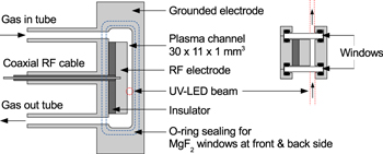
Figure 1. Schematic of the rf plasma source in side view (left) and cross section top view (right). Reprinted from [35], with permission of AIP Publishing.
Download figure:
Standard image High-resolution imageThe investigated plasma source matches closely the key dimensions and properties of an existing well-characterised micro-plasma jet source [33, 59], apart from the up-scaled plasma channel width, here 11 mm instead of 1 mm, thus offering a longer absorption path and lower ozone detection limit; the corresponding surface-to-volume ratios; and the guidance of the exhaust gas through tubes over about 50 cm length into an air extraction, instead of directly into ambient air. In terms of plasma power, the actual electrical power input into the core plasma was measured by a plasma power probe (SOLAYL, Vigilant power monitor, VPM-13.56-1K-1F-1M, Max 1000 W) connected between the matching unit and the plasma source. In comparison with measuring the power output of the rf generator this method excludes unknown power losses within the rf matching network [60] giving a more accurate measure of the plasma power. A comparison between both plasma sources is still possible, since our measurements cover the complete power range from the minimum limit for plasma sustainment to the upper limit just before transition into an unwanted constricted mode, by using those two limits as relative reference points.
2.2. UV-broadband absorption setup and procedures
The ozone density in the core plasma (averaged over the electrode width and the electrode gap distance) was measured by broadband absorption of the corresponding Hartley continuum system ( ) at around λ = 255 nm on the basis of cross-section data [61]. The concept of the experimental setup is to measure the incident and transmitted spectral intensity I0(λ) and IT(λ), respectively, of a beam from a light emitting diode (LED) crossing the absorbing plasma medium through an imaging spectrograph, equipped with a charge coupled device (CCD) camera. This is mathematically reflected by equation (1):
Four different measurements are needed: IPL(λ) the intensity of the light source with plasma on, IL(λ) the intensity of the light source with plasma off, IP(λ) the plasma emission, and IBG(λ) the background signal without light source and plasma. A direct result is the spectral transmission, T(λ), and the absorbance, A(λ), according to Beer–Lambert's law, yielding the averaged absorber density, n, over the line-of-sight absorption length, L, (here 11 mm) for a known absorption cross section σ(λ).
According to [61], the absorption cross section of the Hartley continuum system of ozone exhibits a peak value of 1.17 × 10⁻¹⁷ cm2 within a broad almost symmetrical spectral line shape that is centred at around λ = 255 nm with a full-width at half-maximum (FWHM) of about  = 40 nm. In addition, this cross section has been found to be practically independent of the gas temperature; [52, 62] state a change of about one percent for raising Tg from 202 to 295 K.
The spectrum of the used LED light source is about four times narrower ( = 11 nm), as shown in figure 2. The transmitted intensity spectrum (IT and I0) is recorded with a spectrograph/camera system (described below) that is adjusted to provide a modest spectral resolution of 0.3 nm, which is still sufficient to resolve the product of light source and intrinsic transmission line shapes. Since the line shape of the light source does not fully cover the absorption cross section, spectrally resolved data (measurement and cross section) is required for determining the ozone density according to equations (1) and (2).
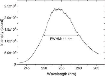
Figure 2. Measured spectrum of the UV-LED.
Download figure:
Standard image High-resolution imageThe two-beam UV-LED absorption setup is in Mach–Zehnder configuration as shown in figure 3. The used UV-LED light source (UVTOP, 255-TO18-FW) provides a spectrum with a centre wavelength of λ = 255 nm and FWHM of  = 11 nm, see figure 2. It is attached to a mounting head that is actively temperature-controlled through a piezo element, and driven by a stabilised current/power supply unit (Thorlabs, LTC100). The typical LED current is 20 mA, the typical optical output power is 150 μW, and the stability of the current supply is specified to be better than 10−4.

Figure 3. Schematic of the two-beam UV-LED absorption setup. The probe beam and reference beam are represented by green-solid line and red-dash line, respectively.
Download figure:
Standard image High-resolution imageAs shown in figure 4(a), the UV-LED is at first imaged 1:1 by an f = 100 mm, ϕ = 25 mm fused silica lens (L1) into the vertically orientated plasma channel, and from there 1:1 with an identical lens (L2) onto the vertically orientated entrance slit of the spectrograph. This represents the probe beam. Additional mirrors (M2), beam-splitters (BS1, BS2), and a third lens (L3) are used to symmetrically couple out a reference beam of similar intensity that by-passes the plasma source.

Figure 4. Illustration of detailed beam paths: (a) top view and (b) side view.
Download figure:
Standard image High-resolution imageThis reference beam is imaged onto the spectrograph's entrance slit and the CCD camera chip, but on a different vertical position due to vertical beam displacement through alignment of BS1 and M2 (see figure 4(b)). Both beams are fully separated by a horizontal blocking cover in front of the entrance slit. The reference beam goes onto the lower half of the CCD chip, rows 0–256, and the probe beam is imaged on the upper part, rows 257–512. The spectrograph's grating disperses the incoming light in the horizontal direction onto 2048 pixel columns which relate to a wavelength range of about 23 nm, see figure 5.
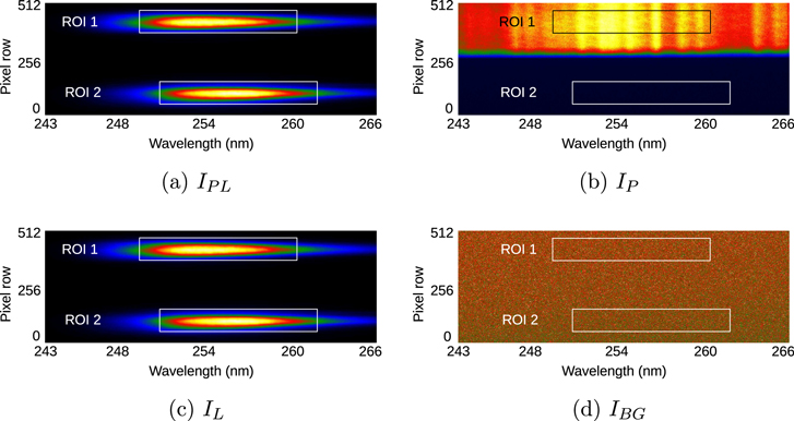
Figure 5. CCD images of the probe beam (pixel row 370–470 (ROI 1)) and reference beam (pixel row 40–140 (ROI 2)) intensities obtained with (a) LED and plasma, (b) plasma only, (c) LED only, and (d) background only. The colours indicate the counts per pixel on a linear colour scale from min-to-max (blue-to-yellow) value, respectively.
Download figure:
Standard image High-resolution imageThe used spectrograph is a 0.5 m-Czerny–Turner imaging spectrograph (Andor, SR-500i) equipped with AL + MgF2 coated optics including a 2400 lines mm−1 grating that is blazed for λ = 300 nm. The grating efficiency is specified to be 65 ± 5% over the relevant spectral range. Attached to the spectrograph is a non-intensified CCD camera (Andor, Newton DU940P-BU2, 2048 × 512 pixels of each the size of 13.5 μm × 13.5 μm) providing high and spectrally constant quantum efficiency of about 60 ± 10% in the relevant observed spectral range, low-noise fast-readout electronics (1 MHz at 16 bit), as well as low dark current due to internal cooling (here −80 °C).
For the ozone broadband absorption measurement the CCD chip samples the vertically separated probe and reference beams within the entrance slit height of 14 mm over a spectral interval from about 243–266 nm, see figure 5. The width of the entrance slit was adjusted to 950 μm resulting in a spectral resolution of 0.30 nm. The beam waist of the LED hitting the plasma device is chosen to have a diameter of about 2 mm, for providing a spatially averaged ozone density measurement across the electrode gap of 1 mm. The spatial resolution along the 30 mm long plasma channel is given by the width of the spectrograph's entrance slit, roughly 1 mm. The required probe beam intensity values (IPL, IP, IL, and IBG) were obtained from the recorded pixel counts within the relevant areas (regions of interest, ROI 1) of the CCD chip after subtracting the corresponding value for the thermal- and readout-noise of the camera that is obtained from the subsequent spectrograph shutter- closed interval, respectively. The ROI was chosen to cover the full spatial beam profile in the vertical direction and the spectral FWHM (11 nm) of the LED in horizontal direction. The corresponding intensity values for the reference beam (I ,
,  ,
,  , and
, and  ) provide additional insight into stability and drifts of the experimental setup. To ensure correct density evaluation according to equation (1), the measured spectra were numerically centred to account for the 2 nm spectral shift of the reference beam with respect to the probe beam on the CCD chip.
Monitoring the probe and reference beam intensities over time allows the stability of the experimental setup to be assessed and the warm-up time and drift of individual components to be identified. In figure 6, after switching-off steady-state plasma operation, IL drifts relatively strongly over time due to changes of conditions in the probe beam pass. The reason was identified as the cooling of the powered electrode temperature from 313 to 294 K (room temperature) over a typical time scale of 30 min, as measured with an infrared thermometer (Precision GOLD, N85FR). In order to suppress this temperature related drift and to reduce the total measurement time, a plasma on/off triggering scheme was chosen, which allows each of the four quantities to be measured within a cycle of 10 s (i.e. short compared to the drift time). This was optimized with reasonable readout time, number of averaging and minimum noise level of the detector. The details are described in the following paragraphs. All density measurements were taken after the warm-up time of the LED and power supply unit of about 30 min, as illustrated in figure 7 in terms of the 'simple' probe beam intensity IL (without plasma).

Figure 6. Probe and reference beam intensities IL and  , IL/I
 ratio and corresponding electrode temperature monitored before and after switching-off steady-state plasma operation.
Download figure:
Standard image High-resolution image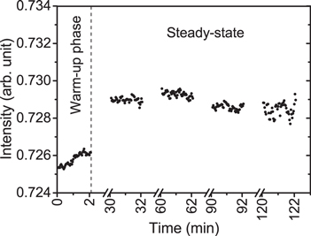
Figure 7. Probe beam intensities IL monitored from switching-on the LED supply/control unit and optical detection system (no plasma).
Download figure:
Standard image High-resolution imageIn order to measure the optical transmission through the plasma in terms of the required four quantities (IPL, IP, IL, and IBG) with correction for the thermal and readout noise of the CCD camera, we make use of four switches: an opto-mechanical shutter for the LED, a TTL input for rf generator on/off operation, an opto-mechanical shutter behind the entrance slit of the spectrograph that blocks all incoming light onto the CCD camera chip, and the camera acquisition trigger input. The temporal triggering scheme is utilised with a four-channel arbitrary function generator (TTi, TGA 12104, 100 MHz sine) and illustrated in figure 8. Note, the shutter behind the slit is ON for a CCD camera chip exposure time of 1.2 s and OFF for the corresponding chip readout time of 1.29 s. The former was chosen to be much longer than the response time of the opto-mechanical switches (typically 10 ms) and the plasma build-up time (a few milliseconds).
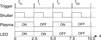
Figure 8. Triggering scheme for measuring the four quantities (IPL, IP, IL, and IBG).
Download figure:
Standard image High-resolution imageIn the steady electrode temperature period, the ratio of both beams, as shown in figure 6, has been taken into account for the determination of the transmission  by the reference beam correction using equation (2):

This additional normalisation with respect to the reference beam intensity significantly reduces the effect of fluctuations in the probe beam intensity on the determination of O3 densities compared to the direct calculation based on one beam only as shown in figure 9. For this example case, at 6.3 W rf plasma power and 10 slm He with 0.1% O2, the O3 density from the one beam direct calculation yields 7.7 ± 3.1 × 1013 cm−3 compared to 7.6 ± 0.9 × 1013 cm−3 from the ratio calculation. Due to the significantly reduced uncertainty, the reference beam correction was used throughout this article for O3 density measurements.
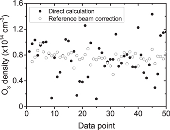
Figure 9. Comparison between 50 data points of O3 density by direct calculation and reference beam correction measured at 6.3 W rf plasma power, 10 slm He with 0.1% O2.
Download figure:
Standard image High-resolution imageA single measurement for each of the four quantities (IPL, IP, IL, and IBG), their reference values and the respective ozone density value according to equation (2) is obtained from one full triggering cycle of 10 s (see figure 8). 50 consecutive measurements for each quantity were recorded and statistically averaged to derive the ozone density data presented.
With the plasma source attached to a three-axis manipulation stage, spatially resolved O3 densities were measured along the 30 mm long plasma channel as shown in figure 10. The O3 density is found to increase from the gas inlet at −30 mm towards the centre at −15 mm. Then, an equilibrium establishes from the centre towards the end of the plasma channel at 0 mm which corresponds to the atomic oxygen equilibrium range found in [58]. All further measurements were taken with the probe beam positioned in the middle of the equilibrium range at −7.5 mm.
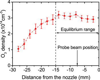
Figure 10. Measured O3 density along the 30 mm long plasma channel, (He-flux 10 slm, O2 admixture 0.5%, rf plasma power 14.5 W).
Download figure:
Standard image High-resolution image2.3. Gas temperature measurements
The same optical detection system (spectrograph and camera in the experimental setup described above) is also used to record optical emission spectra of molecular nitrogen impurities from the centre of the plasma channel. Those spectra are then analysed to deduce the gas temperature. Among the observed spectral features of the N2 (C 3
 B 3
B 3 ) second positive system, see figure 11, we chose the well separated vibrational transition
 with a band head position near λ = 380 nm. A simulated rotational band spectrum on the basis of a thermal population distribution among the rotational sub-levels of the upper N2(C) state is numerically fitted to the measured spectra, as shown in figure 12.
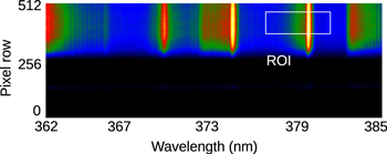
Figure 11. CCD image of the optical emission from the N2 second positive band system. The white rectangular illustrates the chosen region for investigating the υ = 0  2 vibrational transition.
Download figure:
Standard image High-resolution image
Figure 12. Optical emission spectrum of the N2 (C 3
 B 3
B 3 ) (υ = 0
  2) rotational band. The black solid curve represents the measured spectra while the red dot-dash curve represents the result of the spectral fitting simulation; for details see text.
Download figure:
Standard image High-resolution imageThis spectroscopic method is well established, see e.g. [53] and references within, since the high collisionality under atmospheric pressure ensures a full rotational-translation equilibrium. The applied numerical spectra simulation and fitting procedure has successfully been cross-checked against other commonly used software, e.g. LIFBASE, and applied before [28, 63]. In order to conduct the gas temperature measurements, a very small air gas leak in the feed gas tube of the plasma source had to be introduced as an impurity. Its influence was checked to not change the ozone density within the corresponding measurement accuracy. The detection system was operated with a FWHM of 0.29 nm at λ = 380 nm, and with a total camera exposure time of 30 s. The results of the rotational/gas temperature measurements under our experimental conditions exhibit an absolute uncertainty of about ±10 K as a typical deviation between the evaluation of different rotational bands of the second positive system of molecular nitrogen (not shown), but a smaller relative/statistical uncertainty of ±5 K for repeating the measurement or parameter variation.
3. Global model
In order to better understand the production and destruction of reactive species in cold atmospheric pressure plasmas zero-dimensional global models are often employed [64]. Here, the zero-dimensional plasma-chemical kinetics model GlobalKin [55, 56] is used to identify and analyse the production and destruction mechanisms of reactive species within the investigated atmospheric pressure plasma. GlobalKin consists of three modules; a reaction chemistry and transport module, a two-term Boltzmann equation solver for the electron energy distribution function (EEDF), and an ordinary differential equation solver.
GlobalKin calculates absolute species densities accounting for different production and loss mechanisms in the plasma bulk and at the walls bounding the plasma. To describe the plasma-chemical kinetics in the gas phase, the reaction mechanism proposed by Turner [48] for a He/O2 atmospheric pressure plasma is implemented. This is composed of 25 species and 373 chemical reactions. We adopt the heavy particle reaction rates from this mechanism. Different to assuming a Maxwellian EEDF, as in [48], the internal two-term Boltzmann equation solver of GlobalKin is used to calculate the EEDF, and the corresponding electron impact rate and transport coefficients, using electron impact cross sections where they are available. References for the cross sections used in the EEDF calculations can be found in the appendix. This approach has the advantage that the EEDF is self-consistently calculated, and frequently updated during the simulation. Assuming a pseudo-one-dimensional plug flow, the temporally dependent quantities are converted into spatially dependent quantities along the plasma channel by taking into account the gas flow rate and the cross sectional area and length of the plasma source. The total gas flow velocities are chosen to match the lower and upper limits discussed in the experimental section, while the O2 admixture and power are varied as in the experiment.
The loss of particles to the surfaces is treated by diffusion, where the reaction probability is expressed by surface loss coefficients γ and return fractions f. A surface reaction probability denotes the probability that a species reaching the wall reacts with the wall, while the return fraction specifies the fraction of the reacting species which returns to the gas phase as another species.
We assume the surface reaction coefficients to be 1 for positive ions, which denotes neutralisation at the wall. In these cases, ions return as their neutral counter-part with a return fraction f = 1. For ions where the neutral counter-part is not stable (such as  ), the particles are assumed to return as basic fragments (i.e. two O2 molecules in the case of
  ). Electrons are assumed to be lost at the wall, with
  and f = 0. Negative ions typically do not reach the walls due to their inability to cross plasma sheath potential. Therefore, they are given surface reaction probabilities of 0.
Surface reaction probabilities for neutral species are known to be important parameters under low-pressure conditions [65, 66] and typically depend on a number of factors. Limited information exists on the values of these coefficients in atmospheric pressure plasmas where the coverage of surfaces by adsorbed atoms or molecules is likely to be high, meaning that the surface reaction dynamics may differ significantly from those at low-pressure. To account for this uncertainty, simulations were carried out with surface reaction probabilities of 1 and 0 for oxygen containing neutral species. For oxygen atoms surface recombination is assumed with each oxygen atom returning to the gas phase as half an oxygen molecule. It was found that even with a surface reaction probability of 1, the dominant loss processes of these species occur in the gas phase. This is a result of their relatively high masses and low diffusion coefficients at atmospheric pressure, meaning that they do not easily reach the walls of the considered plasma source under atmospheric pressure conditions. However, at low O2 admixtures, surface recombination was found to contribute up to 20% to the total loss of atomic oxygen when its surface loss coefficient was set to 1. This is likely a significant overestimate of the real value, however, it does indicate that surface processes can play some role in determining the density of atomic oxygen under the discussed conditions. However, given the uncertainty in the values of surface reaction coefficients for oxygen containing neutral species we set them to zero for the results presented in this work. Highly reactive He metastables (He(23S) and the molecular state He2( )) have a much lower mass and therefore higher mobility than oxygen containing species. As such, they are assumed to react at the walls with
  and return as one or two ground state He atoms, respectively. However, even with
  the simulation results show that wall losses do not significantly contribute to the total loss of He metastables.
The gas temperature is calculated in GlobalKin through the balance of different heat exchange mechanisms including electron-neutral collisions, exothermic and endothermic chemical reactions, using the heat of formation of the various species, and heat exchange with the surrounding surfaces [55, 56]. Unless otherwise stated, the wall temperatures for different plasma powers are set to the temperature of the powered electrode as measured with an infrared thermometer. These are given in table 1. The electrode temperature was found to remain approximately constant as a function of O2 admixture.
Table 1. Temperature of the powered electrode at different plasma powers, measured with an infrared thermometer.
| Power (W) | 6 | 9 | 11 | 15 | 18 | 21 | 24 | 27 |
| Tw (K) | 298 | 300 | 301 | 304 | 306 | 306 | 307 | 309 |
In order to investigate the main production and destruction pathways for O3, we use the pathway analysis tool PumpKin [67]. PumpKin calculates effective lifetimes of species, where the shortest lived species ('branching point species') have a zero net production. The timescale on which species are considered branching point species is set by the user. In the present work, we investigate the most fundamental formation and consumption pathways for O3. Therefore, the timescale of interest is set to 0, so that branching point species are not considered.
4. Results and discussion
The absorption setup developed in this work for ozone density measurements provides an overall fluctuation level for the unabsorbed baseline signal of about 4 × 10⁻⁴. This limit is mainly determined by changes in the absolute intensity of the UV-LED light source due to the instability of the corresponding current/power supply unit, rather than signal-to-noise limitations of the CCD camera used. An impact of possible spectral fluctuations can be excluded, since we evaluate the UV-LED intensity integrated over its spectral FWHM of about 11 nm, and it fits well within the broader and smooth ozone absorption cross section profile. On the basis of the absorption path length of 11 mm and the absorption cross section data with a maximum value of 1.17 × 10⁻¹⁷ cm2 at λ = 255.5 nm, the corresponding ozone detection limit amounts to 9.0 ± 0.9 × 1013 cm−3. This equals to 3.7 ± 0.4 ppm at atmospheric pressure, which is in the order of bio-technologically relevant concentrations. The growth of E. coli bacteria, for example, was found to retard at ozone concentrations above 4 ppm [68].
This investigation focuses on the discharge operating in homogeneous α-glow-mode over the entire electrode surface at a constant He-flux of 10 slm. The actual rf-plasma power is varied from 6.3 W, required for sustainment, to 25.1 W, just below the limit at which the plasma transits into a constricted mode. The O2 admixture is varied from 0.1% to 0.9%, which is motivated by reports of an atomic oxygen density maximum at around 0.5% O2 [35, 36] and the consequent relevance for technological applications. All density results stated in the following are based on mean average and standard deviation statistical data taken over 50 consecutive samples. Each ozone density measurement is accompanied by a spectroscopic measurement of the gas temperature.
Figure 13 shows the measured ozone density as a function of the rf-plasma power for different O2 admixtures. All these dependencies exhibit a similar shape with decreasing ozone densities towards higher powers. With the same rf-plasma power, the dependence of the ozone density on the O2 admixture is found to be slightly over-linear, as shown in figure 15. The total ozone density increase of about one order of magnitude over the complete range of O2 admixture is comparable with the total increase of the O2 content of a factor of 9. Figure 14 shows the correspondingly measured gas temperature as a function of the rf-plasma power for different O2 admixtures. For all O2 admixtures the temperature shows the expected, approximately linear, increase with increasing rf-plasma power [57].
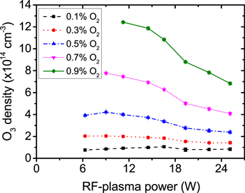
Figure 13. Measured O3 density as a function of the rf-plasma power for different O2 admixtures, He-flux 10 slm.
Download figure:
Standard image High-resolution image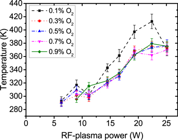
Figure 14. Measured gas temperature as a function of the rf-plasma power for different O2 admixtures, He-flux 10 slm.
Download figure:
Standard image High-resolution imageFigure 15 shows a direct comparison between measured and simulated O3 densities and gas temperatures as a function of O2 admixture at a fixed plasma power of 14.5 W. These results are obtained for the upper limit of the gas flow velocity (lower limit of gas residence time) discussed in the experimental setup section of this work. Changes in O3 and Tg under these conditions are insignificant when taking into account the additional gaps between electrodes and glass windows (lower limit of the flow velocity, higher limit of residence time), and are therefore not shown here. O3 densities are increasing with increasing O2 admixture, and a good qualitative agreement between the experimental and simulation results is observed. As previously obtained by Turner [69], we find that the main net production pathway for O3 is the 3-body recombination reaction of O and O2 and the main destruction pathway is via collisions with O2(b )
)


Both contribute more than 90% to the production and destruction of O3, respectively, within the range of the O2 variation. Reaction (3) is a net-production reaction. In addition to the direct channel, reaction (3) also proceeds via the production and quenching of vibrationally excited O3

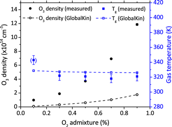
Figure 15. Measured (black filled circles) and simulated O3 (black open circles) density, as well as measured (blue filled squares) and simulated (blue open squares) gas temperature as a function of the O2 admixture, He-flux 10 slm, rf-plasma power 14.5 W. Simulation results are for higher limit of flow velocity as discussed in text.
Download figure:
Standard image High-resolution imageThe quantitative differences between simulation and experiment in figure 15, (factor of 10 at lowest O2 admixture to factor 6 at highest O2 admixture), can be explained by several factors. First of all, a comprehensive sensitivity and uncertainty analysis carried out in other works [48, 69] has revealed that strong coupling between the reaction kinetics of O2( ) and O3 can lead to large uncertainties in the density of O3 in simulations of He/O2 plasmas. In [48], the upper and lower limits of O3 density predicted by the simulation were up to a factor of 13 different in an intermediate regime of O2 admixture (0.3–0.6% O2) due to the strong coupling between the densities of the two species. Furthermore, since the density of O3 is determined by the densities of two transient species (O and O2(
 )), uncertainty in the rate coefficients of production or destruction of either species can significantly influence the uncertainty in the density of O3.
The reaction rate coefficient for both the production (reactions (3) and (5)) and consumption (4) channels are temperature dependent. However, as shown in figure 15, the gas temperature stays approximately constant under a variation of the O2 admixture. Experimental and simulation results for Tg are in very good agreement. It is therefore concluded that the increase in O3 density with O2 admixture is mainly a result of the increasing densities of O (maximum at 0.5%) and O2. This leads to the total production rate increasing more rapidly than the total consumption rate through interactions with O2( ).
).
Figure 16 shows the absolute O3 density and gas temperature as a function of the plasma power, for a constant O2 admixture of 0.5%. Both experimental and simulated O3 densities decrease with increasing plasma power, while the gas temperature increases. A good quantitative agreement is achieved between simulated and experimental gas temperatures. The deviation between measured and simulated gas temperatures occurring at high powers is likely a result of the plasma transitioning into a mixed α/γ mode. In this mode the plasma becomes less homogeneous, an effect which is not captured in the volume-averaged zero-dimensional simulation. The qualitative agreement between experiment and simulation for the O3 densities is good. The quantitative discrepancy is likely a result of the large uncertainty associated with the simulated O3 density under these conditions, as discussed previously.

Figure 16. Measured (black filled circles) and simulated O3 (black open circles) density, as well as measured (blue filled squares) and simulated (blue open squares) gas temperature as a function of the rf-plasma power, He-flux 10 slm, O2 admixture 0.5%. Simulation results are for higher limit of flow velocity as discussed in text.
Download figure:
Standard image High-resolution imageDue to the strong change in gas temperature, the change is O3 densities with power is now affected by both the contribution of gas temperature as well as power. While the gas temperature affects the reaction rate coefficients for both the production and consumption of O3, the power has an impact on the electron density and therefore the production and consumption of O and O2(b ). In order to investigate the contribution of the two influences (gas temperature and power), we manually fix the gas temperature in the simulation to 295 K (room temperature). Simulated O3 densities are shown in figure 17 as a function of power for a self-consistently calculated (blue symbols) and fixed gas temperature (red symbols) for the minimum (unfilled symbols) and maximum (filled symbols) estimated gas flow velocities. The shaded regions therefore represent the variation in the simulated O3 density as a result of different gas flow velocities/residence times as a function of power. This can be viewed as a gauge of the uncertainty in the simulated O3 arising from the estimated gas flow characteristics. O3 densities for different flow velocities deviate more strongly at low powers, since, at low power, the O3 density takes longer to reach steady-state value within the plasma channel. O3 densities simulated with a fixed Tg = 295 K are higher than densities obtained with the self-consistently calculated gas temperatures in GlobalKin, clearly showing an effect of the assumed gas temperature. Additionally, O3 densities are still decreasing with increasing power, despite the fixed gas temperature. Clearly, both temperature and power influence the O3 kinetics. These effects are observed at both the low and high limits of the gas flow velocity.

Figure 17. Absolute experimental (black squares) and simulated (red and blue triangles) O3 densities as a function of plasma power, for a fixed Tg = 295 K, and gas temperature self-consistently calculated in the simulation. Filled symbols and solid lines represent simulation results obtained for the upper limit of the gas flow velocity, as discussed in the experimental section, whereas open symbols and dashed lines represent simulation results for the lower limit of the gas flow velocity. The results for the true gas flow velocity are expected to lie within the shaded areas.
Download figure:
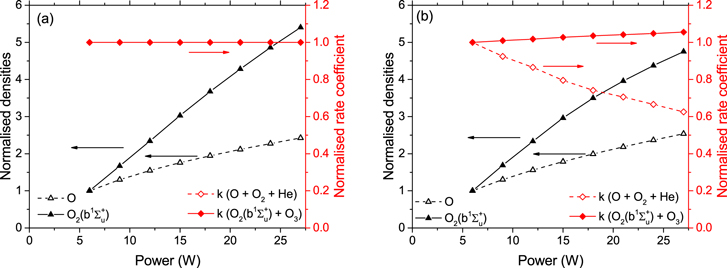
Standard image High-resolution imageFigure 18 shows the normalised O and O2(b ) densities as well as the rate coefficients for production and consumption of O3. The simulation results for the upper limit of the gas flow velocity are used here to illustrate the trends with increasing power, which are similar for the lower gas flow velocity case. Figure 18(a) is for a fixed Tg = 295 K, therefore the temperature dependent rate coefficients do not change as a function of power. Absolute densities of O and O2(b
 ), however, both show a significant increase with power, particularly O2(b
 ), which increases by more than a factor of 5 over the investigated power range. The fact that O2(b
 ) is increasing more strongly with power than O at a constant gas temperature explains the decrease of O3 in figure 17 (red symbols).
Figure 18. Normalised O and O2( ) densities (left axis) and rate coefficients for the production and consumption of O3 (right axis) as a function of power. (a)
  K and (b) self-consistently simulated Tg. In (a) the data points for k (O + O2 + He) coincide with those for k (O2(b
 ) + O3). All data shown is taken from the simulations using the upper limit of the gas flow velocity.
Download figure:
Standard image High-resolution image
Figure 18(b) shows normalised densities and rate coefficients for the self-consistently calculated gas temperatures obtained from the GlobalKin simulations. While the O and O2(b ) densities show approximately the same trends as previously discussed for the fixed-temperature case, the normalised rate coefficients now also show a clear dependence on power, because the calculated gas temperatures increase with power, as shown in figure 16. In particular, the rate coefficient for production of O3 decreases strongly, while the rate coefficient for consumption increases weakly. Both trends lead to a further decrease of O3 densities with power. Therefore, O3 densities obtained with the self-consistently calculated gas temperatures are smaller than O3 densities obtained with a fixed (low) gas temperature, as shown in figure 17. It is therefore concluded that the decrease of O3 with increasing power is a combined effect of an increase in power and gas temperature.
5. Conclusions
A sensitive two-beam UV-LED absorption spectroscopy technique was developed. This allowed for careful system stability tests to determine and rule out effects of non-plasma parameters. The two-beam analysis technique provided a significant improvement of the signal-to-noise ratio by cancelling out fluctuations of the probe beam. This reduced the measurement error by a factor of 2–3 compared to a standard one-beam technique.
This technique enabled sensitive spatially resolved O3 density measurements inside an active plasma channel showing a building-up region transiting into an equilibrium region. Detailed measurements in the equilibrium region were carried out for a non-thermal capacitive 13.56 MHz rf driven atmospheric pressure plasma source with a minimum O3 density of 9.0 ± 0.9 × 1013 cm−3 at 10 slm He with 0.1% O2 admixture, which represents the detection limit by coincidence. The results were correlated to gas temperature measurements, deduced as rotational temperature of the N2 (C 3
 B 3
B 3 , υ = 0
  2) optical emission from introduced small air impurities.
A zero-dimensional plasma-chemical kinetics simulation was applied to interpret the trends in the measured O3 densities. The simulation reveals the mechanisms leading to a decrease in O3 density with increasing power. It was found that the density of O2(b ), responsible for the consumption of O3, increases more rapidly with increasing power than the density of O responsible for the formation of O3. As a result, the density of O3 decreases with power, even when the gas temperature is kept constant. In addition, the increasing gas temperature with increasing rf-plasma power leads to a decrease in the rate coefficient for O3 formation, leading to a further decrease in the O3 density, compared to the case where the gas temperature is held constant in the simulation.
Data management
Data underpinning the figures in this manuscript can be accessed at: https://doi.org/10.15124/868ec862-a4c2-4df4-b14e-c3a4b8070ebd
Acknowledgments
The authors from the University of York acknowledge support from the UK Engineering and Physical Sciences Research Council (EPSRC) through grants EP/K018388/1 and EP/H003797/1. The authors from the Ruhr-Universität Bochum acknowledge support from the German Forschungsgemeinschaft (DFG) in the frame of the package project PAK 'Plasma Cell Interaction in Dermatology'(SCHU2353/3-1). A Wijaikhum acknowledges financial support from the Development and Promotion of Science and Technology Talents Project (DPST), Royal Government of Thailand scholarship. This work has been done within the LABEX Plas@Par project, and received financial state aid managed by the 'Agence Nationale de la Recherche', as part of the 'Programme d'Investissements d'Avenir' under the reference ANR-11-IDEX-0004-02. The authors would like to thank Professor M J Kushner for providing the GlobalKin code used in this work.
Appendix. References for electron impact cross sections used for the He–O2 chemistry:
| Reaction numbera | ΔE (eV)b | Reaction | References |
|---|---|---|---|
| Helium-electron chemistry | |||
| 5 | 0.00 | e + He  He + e He + e |
[70] |
| 6 | 24.58 | e + He  He+ + e He+ + e |
[70] |
| 7 | 19.80 | e + He  He* + e He* + e |
[70] |
| 8 | 4.77 | e + He*  He+ + 2e He+ + 2e |
[71]c |
| Oxygen-electron chemistry | |||
| 12 | 13.62 | e + O  O+ + 2e O+ + 2e |
[72] |
| 13 | 1.97 | e + O  O(1D) + e O(1D) + e |
[72] |
| 14 | 4.19 | e + O  O(1S) + e O(1S) + e |
[72] |
| 15 | 11.65 | e + O(1D)  O+ + 2e O+ + 2e |
[71]c |
| 16 | −1.97 | e + O(1D)  O + e O + e |
as 13d |
| 17 | 9.43 | e + O(1S)  O+ + 2e O+ + 2e |
[73] c |
| 18 | −4.19 | e + O(1S)  O + e O + e |
as 14d |
| 19 | 2.70 | e + O−  O + e + e O + e + e |
[74] |
| 20 | 17.00 | e + O2  O+ + O + 2 e O+ + O + 2 e |
[75] |
| 21 | 12.06 | e + O2   + e + e |
[76] |
| 22 | 8.40 | e + O2  O(1D) + O + e O(1D) + O + e |
[76] |
| 23 | 10.00 | e + O2  O(1D) + O + e O(1D) + O + e |
[76] |
| 24 | 0.00 | e + O2  O2 + e O2 + e |
[76] |
| 25 | 0.02 | e + O2  O2 + e O2 + e |
[76] |
| 26 | 0.19 | e + O2   + e + e |
[76] |
| 27 | 0.19 | e + O2   + e + e |
[76] |
| 28 | 0.57 | e + O2   + e + e |
[76] |
| 29 | 0.38 | e + O2   + e + e |
[76] |
| 30 | 0.38 | e + O2   + e + e |
[76] |
| 31 | 0.75 | e + O2   + e + e |
[76] |
| 32 | 0.98 | e + O2  O2(a O2(a ) + e ) + e |
[76] |
| 33 | 1.63 | e + O2  O2(b O2(b ) + e ) + e |
[76] |
| 34 | 4.50 | e + O2  O2(b O2(b ) + e ) + e |
[76] |
| 35 | 6.00 | e + O2  O2(b O2(b ) + e ) + e |
[76] |
| 36 | 0.00 | e + O2  O + O− O + O− |
[76] |
| 37 | 16.02 | e + O2(a ) )  O+ + O + 2 e O+ + O + 2 e |
as 20e |
| 38 | 11.08 | e + O2(a ) )   + e + e |
as 21e |
| 39 | 7.42 | e + O2(a ) )  O(1D) + O + e O(1D) + O + e |
as 22e |
| 40 | 9.02 | e + O2(a ) )  O(1D) + O + e O(1D) + O + e |
as 23e |
| 41 | −0.98 | e + O2(a ) )  O2 + e O2 + e |
as 32d |
| 42 | 0.00 | e + O2(a ) )  O2(a O2(a ) + e ) + e |
[77] |
| 43 | 0.02 | e + O2(a ) )  O2(a O2(a ) + e ) + e |
as 25e |
| 44 | 0.19 | e + O2(a ) )  O2(a O2(a ) + e ) + e |
as 26e |
| 45 | 0.19 | e + O2(a ) )  O2(a O2(a ) + e ) + e |
as 27e |
| 46 | 0.38 | e + O2(a ) )  O2(a O2(a ) + e ) + e |
as 29e |
| 47 | 0.38 | e + O2(a ) )  O2(a O2(a ) + e ) + e |
as 30e |
| 48 | 0.57 | e + O2(a ) )  O2(a O2(a ) + e ) + e |
as 28e |
| 49 | 0.75 | e + O2(a ) )  O2(a O2(a ) + e ) + e |
as 31e |
| 50 | 0.65 | e + O2(a ) )  O2(b O2(b ) + e ) + e |
[77] |
| 51 | 3.52 | e + O2(a ) )  O2(b O2(b ) + e ) + e |
as 34e |
| 52 | 5.03 | e + O2(a ) )  O2(b O2(b ) + e ) + e |
as 35e |
| 53 | 3.50 | e + O2(a ) )  O + O− O + O− |
[78] |
| 55 | 15.37 | e + O2(b ) )  O+ + O + 2 e O+ + O + 2 e |
as 20e |
| 56 | 10.43 | e + O2(b ) )   + 2e + 2e |
as 21e |
| 57 | 6.77 | e + O2(b ) )  O(1D) + O + e O(1D) + O + e |
as 22e |
| 58 | 8.37 | e + O2(b ) )  O(1D) + O + e O(1D) + O + e |
as 23e |
| 59 | −1.63 | e + O2(b ) )  O2 + e O2 + e |
as 33d |
| 60 | −0.65 | e + O2(b ) )  O2(a O2(a ) + e ) + e |
as 50d |
| 62 | 0.00 | e + O2(b ) )  O2(b O2(b ) + e ) + e |
[77] |
| 63 | 0.19 | e + O2(b ) )  O2(b O2(b ) + e ) + e |
as 26e |
| 64 | 0.19 | e + O2(b ) )  O2(b O2(b ) + e ) + e |
as 27e |
| 65 | 0.38 | e + O2(b ) )  O2(b O2(b ) + e ) + e |
as 29e |
| 66 | 0.38 | e + O2(b ) )  O2(b O2(b ) + e ) + e |
as 30e |
| 67 | 0.57 | e + O2(b ) )  O2(b O2(b ) + e ) + e |
as 28e |
| 68 | 0.75 | e + O2(b ) )  O2(b O2(b ) + e ) + e |
as 31e |
| 69 | 2.87 | e + O2(b ) )  O2(b O2(b ) + e ) + e |
as 34e |
| 70 | 4.37 | e + O2(b ) )  O2(b O2(b ) + e ) + e |
as 35e |
| 71 | 0.00 | e + O2(b ) )  O + O− O + O− |
as 36e |
| 75 | 0.00 | e + O3   + O + O |
[79] |
| 76 | 0.00 | e + O3  O2 + O− O2 + O− |
[79] |
aNumbers correspond to reaction numbers in [48]. bGain or loss in electron energy associated with reaction. cCross sections are calculated using expressions in cited reference. dSuperelastic cross section obtained by detailed balance from the corresponding excitation process. eCross section estimated by shifting and scaling the corresponding cross section for the ground state process by the excitation threshold of the excited state.