Impact of Starch from Cassava Peel on Biogas Produced through the Anaerobic Digestion Process


School of Mechanical & Manufacturing Engineering, Dublin City University, Dublin 9, Ireland
*
Author to whom correspondence should be addressed.
Energies 2020, 13(11), 2713; https://doi.org/10.3390/en13112713
Submission received: 24 April 2020
/
Revised: 15 May 2020
/
Accepted: 20 May 2020
/
Published: 28 May 2020
(This article belongs to the Special Issue Selected Papers from SDEWES 2019 conferences on Sustainable Development of Energy, Water and Environment Systems)
Abstract
:Cassava is a form of food that is rich in starch abundant in many countries. Several bio-products can be extracted from its starch and used as an alternative for oil-based products. This study primarily aims to investigate the influence of the starch isolated from cassava peel on the quantity and quality of the biogas produced via anaerobic digestion. Beating pre-treatment was applied for the first time to isolate the starch and mechanically pre-treat the substrate. The influence of temperature, volatile solid and sludge quantity investigations were analysed with the aid of Design of Experiments (DOE). An optimisation process was applied in calculating the energy balance at the optimal results and this was needed in evaluating the impact of the starch on the biogas produced. The study revealed that the influence of the starch on the biogas quality is quite low and, as such, negligible. The largest biogas volume as obtained was 3830 cc at 37 °C, 4.2 g-VS and 50% sludge quantity, while at the same time the maximum CH4 g−1-VS was 850 cc g−1-VS at 37 °C, 1.1 g-VS and 50% sludge quantity. The optimal results show the energy gain could be achieved based on the set criteria.
1. Introduction
The negative impacts of fossil fuels on the environment and the ever-increasing price in energy is driving the conversion to sources of renewable energy more than any time before [1]. The estimated amount of unconsumed human food accounts for about a 33% [2], at a value of approximately 750 billion dollars [3]. Approximately 7% of the harmful emissions of gases result from these quantities of food surplus [4,5]. Waste disposal has become crucially important with excess organic substances becoming useful products in the production of biogas through the anaerobic digestion process [6]. These wastes are often disposed of without treatment, leading to increased environmental pollution [7].
Cassava is becoming a staple food in many regions of the world and, in particular, it is also a known tropical plant that grows in many of these countries, such as in Asia, Africa and South America, and in low-fertility soils [6,8]. Worldwide, over 200 million metric tons were produced from cassava in 2015, hence it is considered as one of the most important food sources that is rich in carbohydrates [7]. For example, 2018 cassava yields rose by almost three-fold to reach 550 million metric tons; about 350 million metric tons comprises cassava waste (peel, leaf, bagasse and stem) [9]. About a quarter of cassava plant waste are peel, leaves and starch residues [10]. Approximately half a ton of cassava peel and pulp produced per ton of processed cassava is used to produce ethanol and starch in some Asian countries, such as Indonesia and Thailand [7,11]. Cassava peel (CP) richness in carbon represents up to 30% of cassava wet weight [12]. Many products can be produced from CP, and as a result has raised itself an interest to researchers for further findings due to its richness in starch [13]. In fact, one of the uses of CP has been in the production of biogas and bio-fertilizer by the anaerobic digestion (AD) process [14].
AD is an energy production process that requires the procession by microorganisms under anaerobic conditions. Various waste types, including household waste, agricultural waste and chemical waste, are processed to produce biogas using several techniques or by the integration of several methods. The amount of energy resulting from the treatment of this waste can reach 1200 kW depending on the waste type and the treatment method used. AD produces biogas-containing methane that can be converted to renewable energy and thus reduces the greenhouse gases [15]. Biogas production from the AD process goes through several steps: hydrolysis, acidinogenic, acetogenic and methanogenic. AD results in biogas, which contains methane under appropriate condition of 60–70% [16] and the residual can be used as bio fertilizer (organic residues rich by nitrogen) [17]. The biogas can be directly used to produce electricity and heat or converted to bio-methane to be used as vehicles fuel [18]. It is one of the effective energy production methods that are used in many countries in Asia and Europe. Operating temperature (psychrophilic, mesophilic and thermophilic), reactor design (plug-flow, complete-mix, and covered lagoons), and solid content (wet versus dry) have an effect on gas resulting from the AD process [17,19]. AD is considered as one of the common processes for the production of biogas from waste in the UK [5].
Biogas was produced from CP without starch extraction in several studies [20,21]. Biogas was produced from CP with urea as a supplement with different concentrations [21]. Biogas was produced from CP at several temperatures and retention time. The maximum production of biogas from the CP at a temperature of 35 °C was after 30-days of retention time [20]. In this study, CP was extracted before the AD process and the retention period was reduced to 21 days instead of 30 days. The purpose of these is to exploit the starch to produce additional bioproducts and to reduce the total costs of the biogas production process. Moreover, the optimisation process was carried out in the study to calculate the energy balance of the optimal results.
The main objective of this study is to investigate the impact of starch isolated from the CP on the quantity and the quality of the biogas produced from the CP. A secondary objective of the study is to confirm the content of the resulted digestate to the three main nutrients of conventional fertilizer (N, P and K). Beating pre-treatment as a mechanical pre-treatment process was applied in the study by employing the Hollander beater for first time to isolate the starch and pre-treat CP followed by AD to produce biogas and methane.
2. Material and Methods
2.1. Substrates and Sludge
Costa Rican Cassava was purchased from Veg-ex shop, Dublin, Ireland. The cassava was peeled manually and cut into small pieces to facilitate the treatment process. A volume of 2.22 kg of cassava peel (CP) was treated by a beating pre-treatment process with a Holland beater for five minutes with 20 L of water. The starch has been isolated from the mixture, dried and then stored for future use. The feedstock was distributed in three containers and the volatile solid (VS) of each container was adjusted to 4.2, 2.65 and 1.1 g-VS.
The sludge was collected from Green Generation Ltd., Nurney, Co. Kildare, Ireland in a 20 L container. The sludge was brought on the same day of the experiment to maintain its properties and to keep it intact from contamination. Total solid (TS) of the sludge was 6.5%, the volatile solid was 4.51% and pH was 8.1.
2.2. Response Surface Methodology (RSM)
Box–Behnken design (BBD) with three numeric factors was conducted in this study. The studied factors were temperature, volatile solid concentration and sludge quantity. They were designed via RSM to describe and evaluate the performance of the process and to also provide the optimal combinations and results. RSM identifies the relationships between the resultant responses and the input variables. The levels of each factor were set as shown in Table 1. The ranges of the three factors were set based on carrying out a number of preliminary trials and in accordance with previous studies [22,23,24]. The results were statistically analysed using Design Expert software (Ver.12, StatEase, Godward St NE, Suite 6400, Minneapolis, MN 55413). The interaction, perturbation between factors and responses and the adequacy of the process were determined by the analysis of variance (ANOVA). The statistical significance of the models developed and each term in the regression equation were also tested using the sequential lack-of-fit test and F-test. The confidence level (95%) of the model ( = 0.05) was tested by the p-value.
2.3. Beating Pre-Treatment
Beating pre-treatment was employed in the study using a Hollander beater device. A volume of 2.22 kg of CP with 20 L of water with ratio 1:9 was placed into the beater for five minutes. This was done to slice the CP into small slices and isolate the starch from the peel. Beating pre-treatment was applied immediately after slicing the feedstock by high-pressure beating against inclined blades. The mixture was discharged into a large container through a sieve to isolate the cassava peel from the mixture. It was left for 3–4 h for the starch to settle down in the container. The water at the top was decanted off and added to the pre-treated peel.
2.4. Total Solid and Volatile Solid
The TS and volatile solid were measured and adjusted as designed in the experiment matrix according to the standard methods (NREL/MRI LAP 1994, 2008) [25]. Three samples were taken directly from the beater (prior to starch separation). Three other samples were also taken after starch isolation to measure the TS and volatile solid. The samples were dried in a drying oven at 105 °C for 24 h to calculate the moisture content (MS) and the TS. Thereafter, the samples were burned at 575 °C for four hours to calculate the ash weight and thus the volatile solid amount. According to previous studies [22,23,24], the preliminary trials which were conducted to set the ranges of the volatile solid (1.1–4.2 g-VS were found to be ideal). The preliminary trials revealed that volatile solid values higher than 4.2 g-VS could lead to a system failure, while lower values of volatile solid leads to a starving condition [26].
2.5. Anaerobic Digestion (AD)
Water was added to each container at a different ratio based on previous studies and the preliminary trials to adjust the value of volatile solid in each container [22,23,24]. The ratio of water to CP was 9:1,18:1 and 27:1, respectively. Volatile solid value of each container was 4.2, 2.65 and 1.1 g-VS. 500-millilitre glass flasks were filled with CP and inoculum at different ratios. Table 1 shows the variable matrix and levels in actual values.
The sludge quantity (SQ) varied in each flask (50%, 37.5% and 25%) of the total volume of 400 mL of the flask. The remainder of the 400 mL was filled with pre-treated CP after were mixed well to ensure that the solids were not deposited at the bottom of the container. The samples that contained starch were used as controls. The same procedure was followed with the controls. In order to allow comparison with the predicted values at the same conditions, the controls were digested at the volatile solid of 4, SQ of 50% and at each of three temperature levels. However, the ratio of water to CP varied due to the presence of starch. The ratio of water to CP in the control samples were 5.75:1, 9.7:1 and 23:1, respectively. Each sample was connected to an aluminium gasbag and the nitrogen pumped into the system and pulled out twice to ensure that the system was free of oxygen. Each sample was conducted in triplicate. The control samples conditions are shown in Table 2. Samples were placed in the water baths at mesophilic operation temperatures (34 °C, 37 °C and 40 °C). The incubation time was 21 days. The flasks were shaken on daily basis over the period of the experiment. The biogas produced from each sample was measured twice (on day 9 and day 21). Biogas volume was measured using volumetric flask. It uses gas-sampling tubes that were installed in a gas jar with confining liquid. A biogas analyser (biogas5000 Geo-tech) was used in the measurement of the concentration of the gases: methane (CH4), carbon dioxide (CO2), oxygen (O2) and hydrogen sulfide (H2S). The pH of the digestate resulted from each sample as measured by Hanna precision pH meter (accuracy ± 0.01), model pH 213 and examined to confirm the suitability of its application in agricultural settings. Figure 1 illustrates the flowchart of the experimental work of the study.
2.6. Energy Balance
The energy balance of the digestion process was calculated by applying the following formulas based on the optimisation results [25]:
Bs = (CH4%) × (9.67)
Ep = Bp × Bs
Ec = Ept⁄VSm
Net Ep = Ep − Ec
Energy balance% = (Net Ep − Ec)/Ec
While the CH4% is the average of methane percentage of each sample, the value 9.67 is a reference value that indicates the energy quantity of 1 Nm3 of biogas [27]. The energy gain in percentage is the difference between the energy gained by the biogas produced from CP (Ep) and the energy consumed in the digestion process (Ec). When the energy gain% is negative, it indicates that the AD process of CP caused a loss of energy.
3. Results and Discussion
3.1. General Results
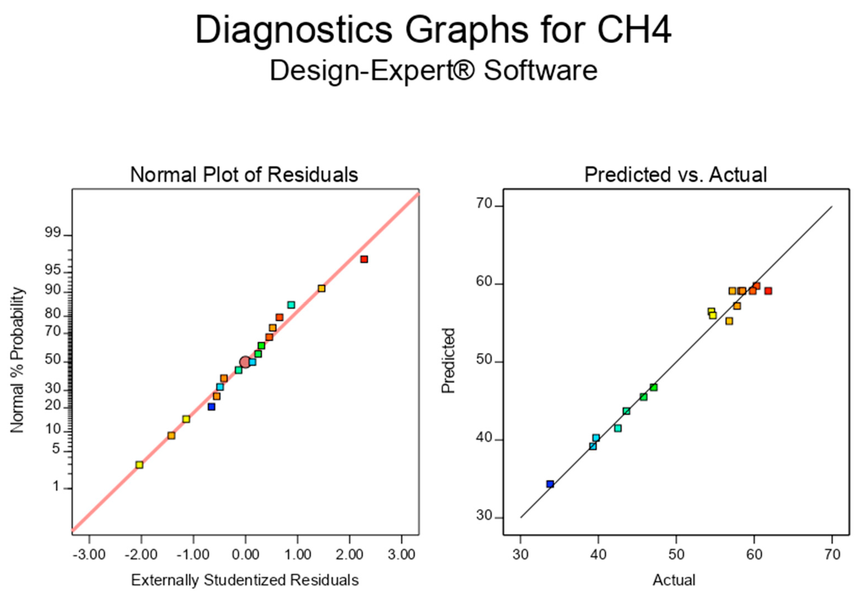
The p-value of all models indicated the models were significant. There is only a 0.01% chance that an F-value this large could occur due to noise as the p-value < 0.0001 for all responses, as shown in ANOVA tables. Additionally, from the same tables, it can be seen that the lack of fit F-value implies that the lack of fit is not significant relative to the pure error for all responses. The impact of each factor, the interaction between factors and the checked probability ("p-value") of the model are described in ANOVA tables. These tables illustrate significant model terms. The tables also show that the all models were adequate as all values of R2, predicted R2 and adjusted R2 were close to 1. For all models the predicted R2 was in reasonable agreement with the adjusted R2 as the difference between them is less than 0.2. The model graphs help in illustrating the behaviour of each response as the factors vary. Since all points are close to the distribution line, this indicates that the distribution was normal and that the adaptation of the model was adequate as shown in Figure 2 and Figure 3, which show the normal probability and predicted volatile solid actual residual figures. As the majority of the points were around the line, the agreement between the actual and predicted response was excellent.
In the coded models the factors are symbolised by letters A, B and C, while in the actual models the factors names are used. The coefficient of the factors in the coded model illustrates the effect of each factor and the greatest effect of any factor is for the factor with the largest coefficient. In the meantime, the coefficient sign indicates whether the effect is positive or negative. A positive sign means an upward effect and a negative sign means the opposite. Additionally, the actual models can be used to predict the response at given factor levels within their ranges used in this study.
The perturbation plots help in determining the influence of each factor on the response of interest, while the effect of the interaction between factors on the responses are illustrated in the interactions figures. Interaction occurs when one factor depends on another factor. This is indicated in the plots by two non-parallel lines. The contour plot is a 2-D graph that illustrates all points that have the same responses and connecting them by contour lines.
3.2. CP Results
Cassava peel constitutes approximately 20–25% of cassava weight, which corresponds to what is mentioned in the study of Eziekiel and Aworh [13]. According to a study in 2018, 5% of the cassava weight is peel. This percentage can be raised to 20% by efficient peeling [28]. In contrast, the current study found that starch represents between 17% and 20% of the CP. This is less than half of what Sivamani et al. mentioned in 2018 [29].
Furthermore, the experimental works of the study revealed that the effect of starch on the quantity of the biogas produced from the AD of CP was relatively low, which ranged between 1% and 3.5%. However, the difference between methane percentages did not exceed 0.66%. Table 3 and Table 4 show the results of all experiment responses and the comparison between actual and predicted values of the control samples.
The highest biogas amount achieved was 3380 cc at 37 °C, 4.2 g-VS and 50% sludge and, in the same run, the concentration of the CH4 and CO2 were 39.3% and 35.7%, respectively. On the other hand, the lowest amount of biogas produced was 831 at the lowest temperature, lowest volatile solid value and 37.5% of sludge, while the CH4 concentration resulting from this run was 56.8% and 19.6% of CO2. The highest percentage of the biogas yield per g-VS was 1442.5 cc g-1-VS, achieved at 40 °C, 1.1 g-VS and 37.5% of sludge. In addition, the lowest volume of the biogas g−1-VS achieved was 479.7 cc g−1-VS at 34 °C, 2.65 g-VS and 25% of sludge.
Moreover, there was an inverse relationship between the percentage of the CH4 resulted and CO2. Based on Table 3, the CH4 percentages ranged from 33.8% to 61.8%. The lowest percentage of CH4 and the largest CO2% were found in run 14 at 37 °C, 4.2 g-VS and 25% sludge, while the highest CH4% was 61.8% at 37 °C, 2.65 g-VS and 37.5% of sludge and the highest CH4 g−1-VS produced was 850.8 cc g−1-VS at 37 °C, 1.1 g-VS and 50% sludge. In contrast, at 34 °C, 4.2 g-VS and 37.5% sludge, the CH4 g−1-VS was 214.9 cc g−1-VS which was the lowest yield. The pH value ranged between 7.7 and 8 for all samples.
Additionally, the actual and predicted values for the control samples were illustrated in Table 4. It highlighted the difference between the percentages of biogas g−1-VS; it reached the peak of −5.3% at 37 °C. The maximum reduction in the CO2 amount was −1.74% at 37 °C. The difference between CH4 g−1-VS values was the highest, as it reached 13.7% at 34 °C and 12.4% at 40 °C while it was 3.9% at 37 °C.
The highest biogas yield of the study on the production of biogas from CP with urea under mesophilic conditions was 80.79 cc g−1-TS. The CP was treated by soaking in water for seven days. The study concluded that the 0.01 of urea with CP increases the biogas volume by 24.33% [21]. Jekayinfa and Scholz [20] found that the highest biogas volume and methane content volume produced from cassava peel were 660 cc g−1-VS and 280 cc g−1-VS respectively at 35 °C. Compared to the previous studies, the results of the proposed study showed an increase in the volume of biogas produced. This increase confirms the potential benefit of treating CP with beating pre-treatment. The study also revealed that there was no obvious impact of the isolated starch on the quantity and quality of the biogas produced.
When comparing the volume of produced biogas from the control samples with the studies described above, the increase in the volume of biogas reached to 4.5%. This could potentially be an illustration of the positive effect of beating pre-treatment of CP, while the ratio decreased to 1% when compared with other samples (starch-free samples), which confirms the limited effect of starch on the resulting biogas. The use of starch in producing more bio-products, such as bio-plastic and bio-adhesive material, could enhance the efficiency of the AD process and increase reliance on it in the future.
3.3. Model Estimation
ANOVA Table 5, Table 6, Table 7, Table 8 and Table 9 for each response show that all developed models were significant. The coded equations (6, 8, 10, 12 and 14) and the actual equations (7, 9, 11, 13 and 15) are shown below with each response. The influences of volatile solid (B) and sludge quantity (C) were significant on all responses, while there was no significant influence of temperature (A) on the CH4 and CO2%. The main effect of the temperature on CH4% and CO2%, which is insignificant, was forced into the model to support hierarchy as presented in ANOVA Table 7 and Table 8. The interaction of (BC) had a significant influence on the CH4, CO2 and CH4 g−1-VS responses. In contrast, the biogas g−1-VS and CH4 g−1-VS are significantly affected by the interaction of temperature and volatile solid (AB). There is no significant influence for the interaction between the temperature and the amount of the sludge (AC) on all responses.
3.3.1. Biogas
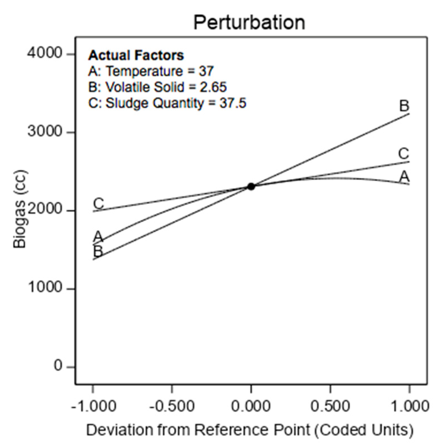
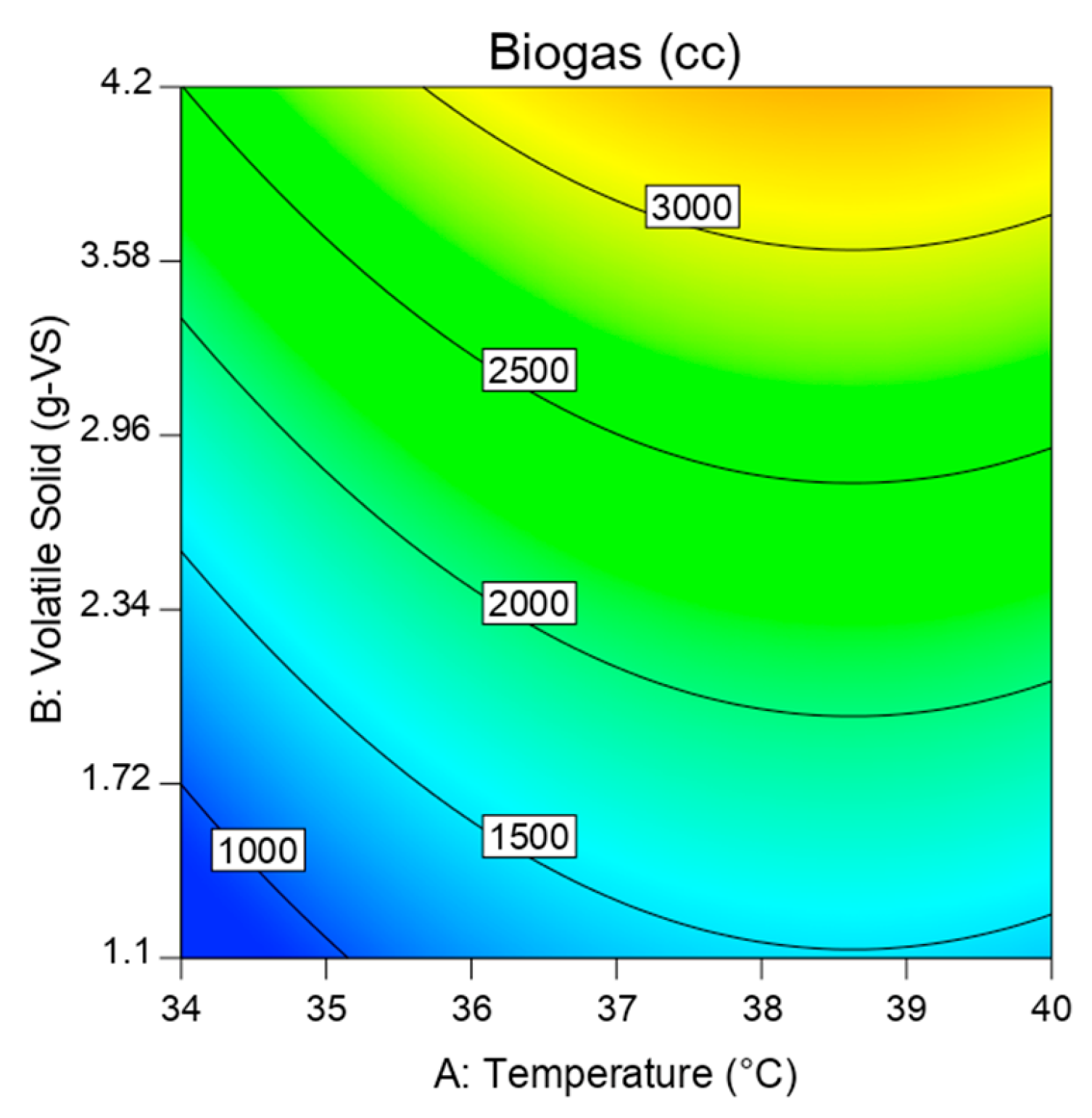
As shown in Figure 4 the highest biogas was achieved at volatile solid of 4.2 g-VS. The figure also shows the direct proportions between the three factors and the biogas produced. These results correspond to several studies about the AD of cassava. In a study of AD of cassava with sludge, it was found that the volume of biogas increased slightly when shifting from the mesophilic condition to thermophilic condition [22]. Panichnumsin found that the yield of methane increases with increasing volatile concentration [23]. The effect of temperature remains directly until it reached to around 38 °C after that it became steady before it reduced slightly. The highest biogas volume when the sludge quantity at 37.5% was at a temperature between (36–40) °C and volatile solid of 4.2 g-VS as clear from Figure 5. The coded Equation (6) clarifies that the highest positive influence of volatile solid on the biogas followed by temperature and sludge quantity:
Biogas = 2310.11 + 389.13 A + 933.75 B + 317.38 C − 359.24 A2
Biogas = −59,681.43752 + 3083.42747 Temperature + 602.41935 Volatile Solid + 25.39000 Sludge Quantity − 39.91512 Temperature2
3.3.2. Biogas g−1-VS
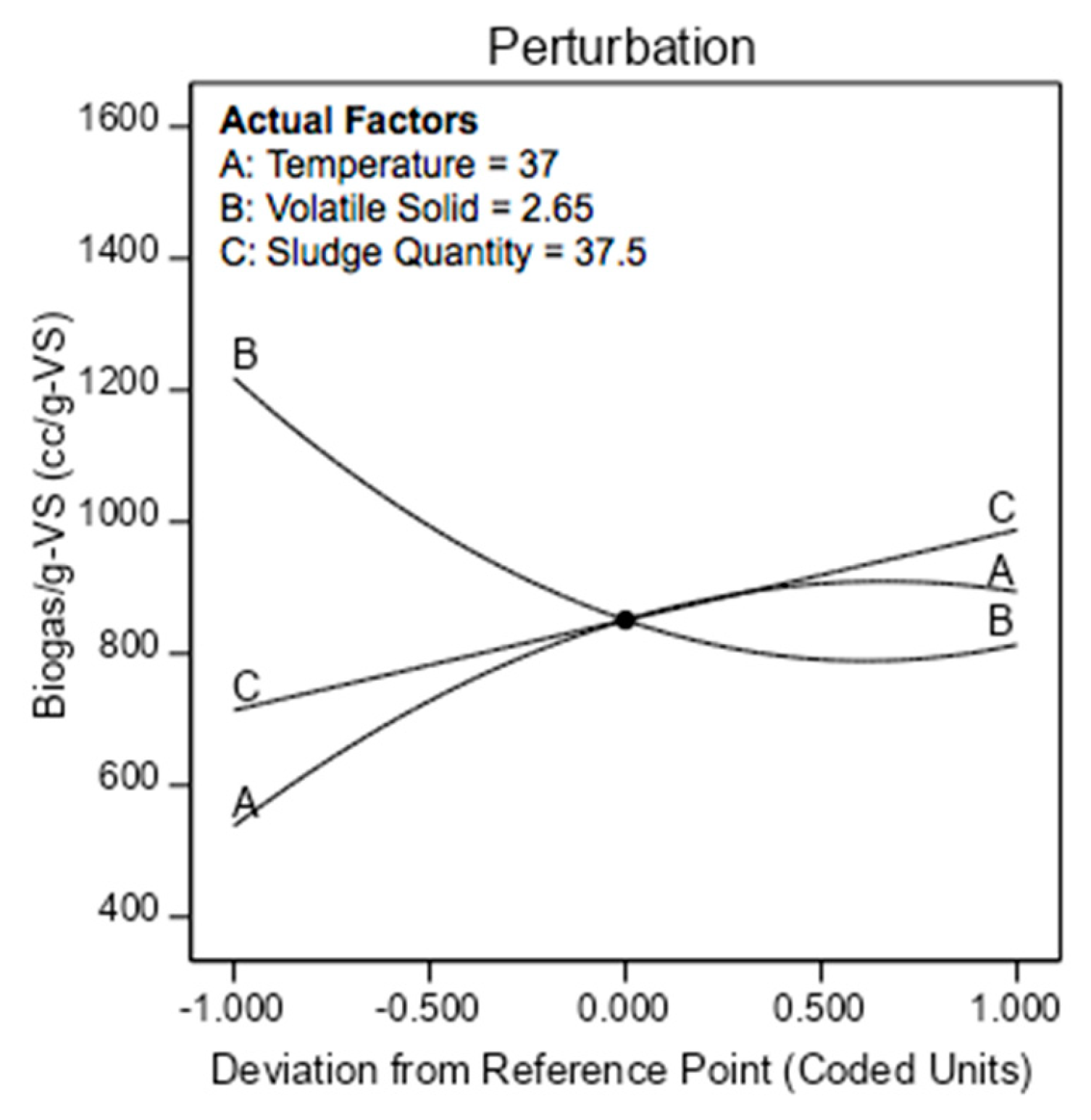
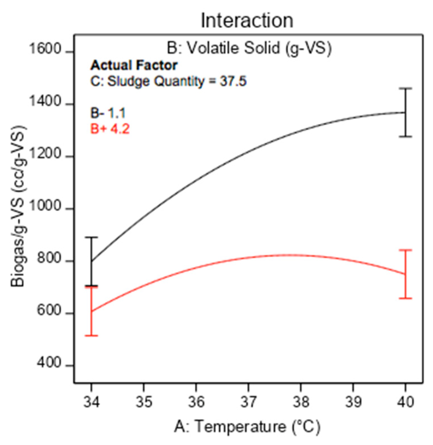
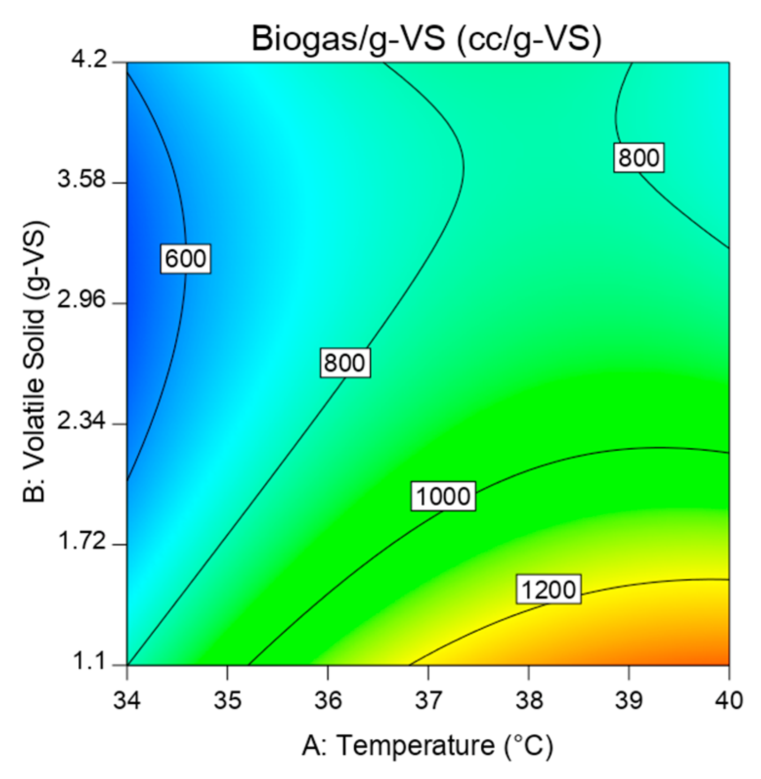
It is evident from Figure 6 that the highest biogas g−1-VS produced was at lowest volatile solid amount of 1.1 g-VS. That is because, when calculating the biogas g−1-VS, the biogas volume divides the volatile solid value: the higher the volatile solid value, the lower the biogas g−1-VS results, and vice versa. In contrast, the same figure illustrates the direct relation between biogas g−1-VS and both of temperature and sludge quantity. As with the biogas impacts above, the effects of temperature stay directly until it reached 38 °C, then it became steady before it reduced slightly. The interaction impact of temperature and volatile solids on the biogas g−1-VS is shown in Figure 7. The response increased slightly by increasing the temperature when using volatile solids of 4.2 g-VS. In contrast it significantly increased when using volatile solids of 1.1 g-VS. The response was in it is minimum values at 34 °C, noting that there was no significance difference when using both volatile solid values. This is due to the fact that the high volatile solid values of cassava requires higher temperatures to fully digest [22]. The contour graph in Figure 8 illustrates the highest biogas g−1-VS was found at volatile solid less than 1.3 g-VS and temperature between 38 and 40 °C. The coded Equation (8) clarifies the highest negative effect of volatile solid on the biogas g−1-VS:
Biogas g−1-VS = 850.98 + 178.04 A − 202.53 B + 136.81 C − 106.80 AB − 134.90 A2 + 165.17B2
Biogas g−1-VS = −23,698.37993 + 1229.40976 Temperature + 354.76907 Volatile Solid + 10.94500 Sludge Quantity − 22.96774 Temperature × Volatile Solid − 14.98918 Temperature2 + 68.75021 Volatile Solid2
3.3.3. CH4%
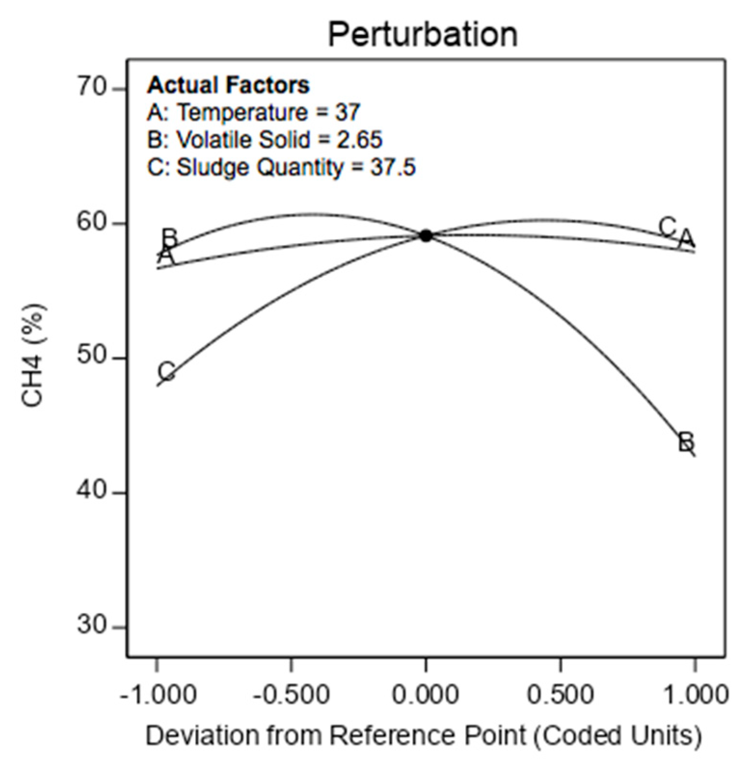
From Figure 9, it can be noted that the influence of temperature was quite low on the methane percentage. Volatile solids slightly positively affect the methane percentage and then decreases dramatically by increasing the volatile solid value. On the contrary, the effect of the sludge quantity positively affects the response and decreases slightly at sludge quantity of 38.5%. Figure 10 shows the influence of the interaction of volatile solid and sludge quantity on the response. The CH4% significantly increased when changing the sludge quantity from 43% to 60%. This is because the promoting of inoculum to the AD process consequently affects the activity of bacteria to increase the methane yields [22,30,31]. The lowest CH4% was found at 4.2 g-VS and both sludge quantities. The contour plot in Figure 11 illustrates the wide area for the highest CH4% achieved when using volatile solids less than 2.5 g-VS and sludge quantity of 37.5% and more. The highest effect on the methane percentage was the volatile solid value followed by sludge quantity as demonstrated in coded Equation (10). The volatile solid negatively affects the response while the sludge quantity positively affects it.
CH4 = 59.12 + 0.6125A − 7.49B + 5.23C − 2.80BC − 1.82A2 − 8.92B2 − 5.95C2
CH4 = −322.49969 + 15.18917 Temperature + 20.27206 Volatile Solid + 3.65577 Sludge Quantity − 0.144516 Volatile Solid × Sludge Quantity − 0.202500 Temperature2 − 3.71384 Volatile Solid2 − 0.038064 Sludge Quantity2
3.3.4. CO2%
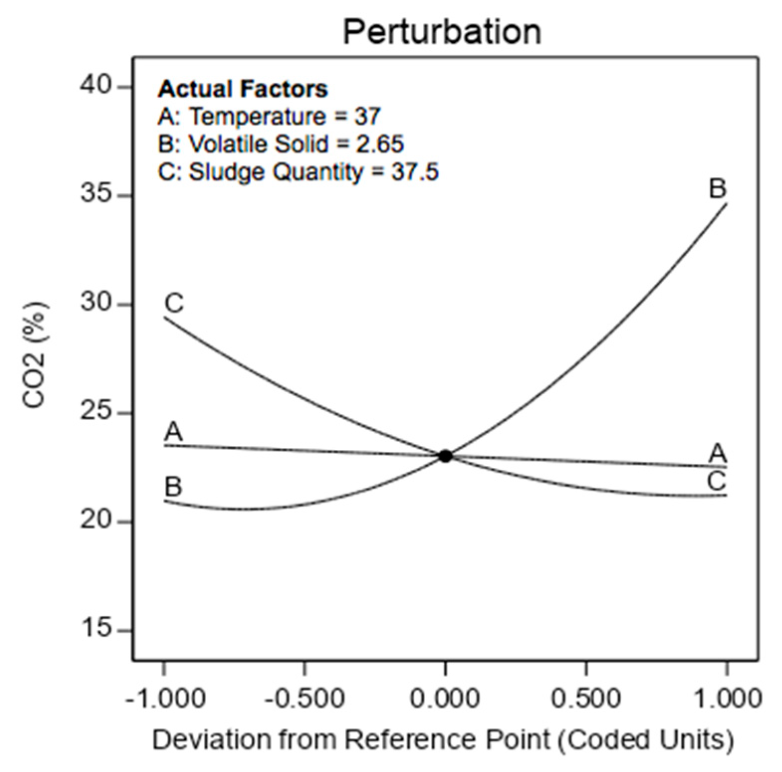
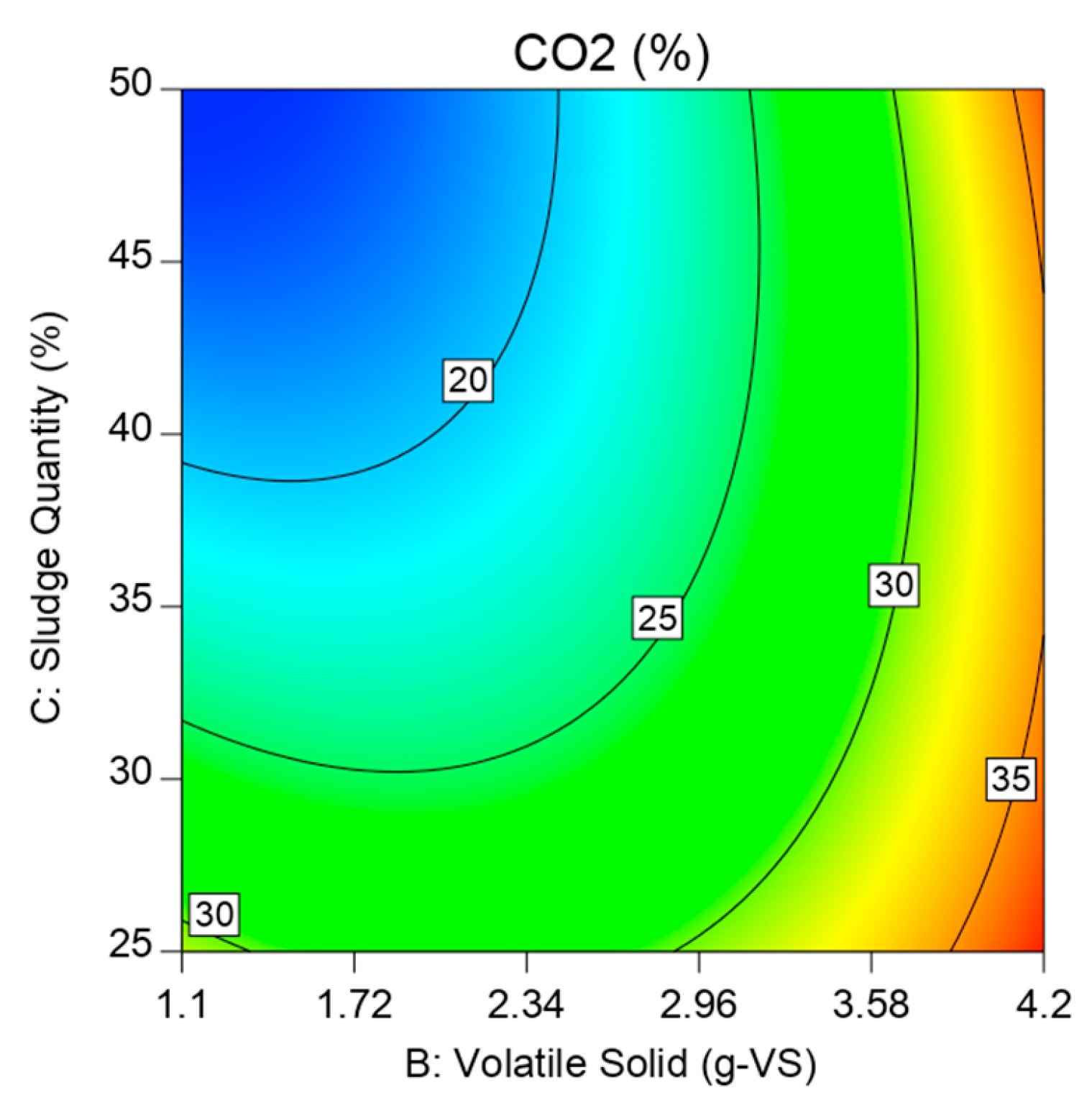
The impact of temperature was quite low on the CO2% as it obvious in Figure 12, whereas it increased significantly by increasing the volatile solid and decreasing the sludge quantity as shown in the same figure. The response slightly increased by increasing the volatile solid at sludge quantity of 25% as clarified in Figure 13. In contrast, CO2% rises rapidly with the increasing of volatile solids at a sludge quantity of 50%, noting that there was no difference in CO2% when using volatile solid of 4.2 g-VS and both sludge quantities. Figure 14 demonstrates the lowest CO2% achieved at the same wide area where the highest CH4% was found, which illustrates the inverse relationship between CH4% and CO2%. Coded Equation (12) shows the positive highest effect of the volatile solid value on the response, followed by the negative effect of the sludge quantity:
CO2 = 23.04 − 0.5000A + 6.85B − 4.10C − 0.9500AB + 3.50BC + 4.79B2 + 2.29C2
CO2 = 62.34837 + 0.374731 Temperature − 5.36725 Volatile Solid − 1.90692 Sludge Quantity − 0.204301 Temperature × Volatile Solid + 0.180645 Volatile Solid × Sludge Quantity + 1.99463 Volatile Solid2 + 0.014669 Sludge Quantity2
3.3.5. CH4 g−1-VS
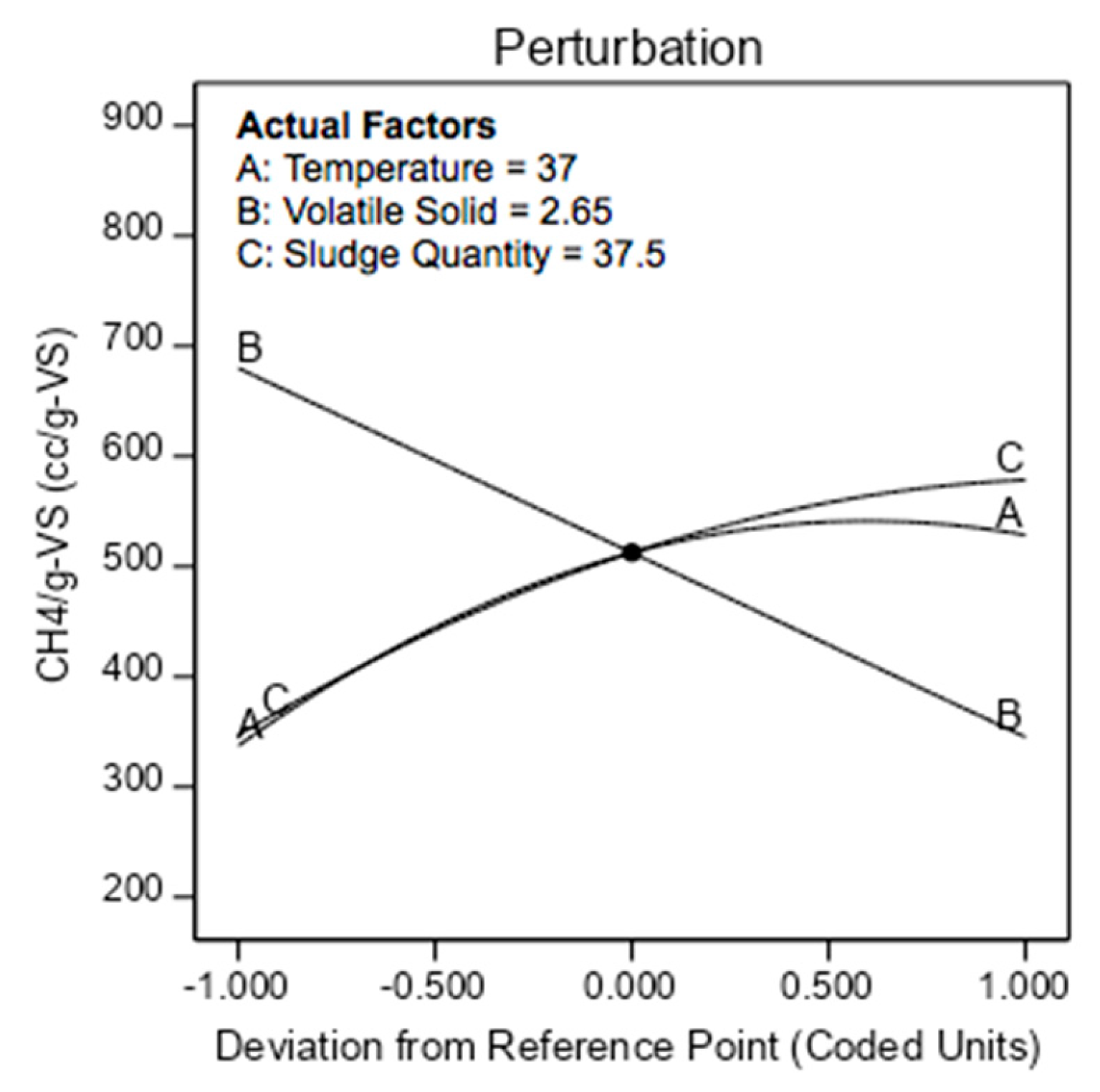
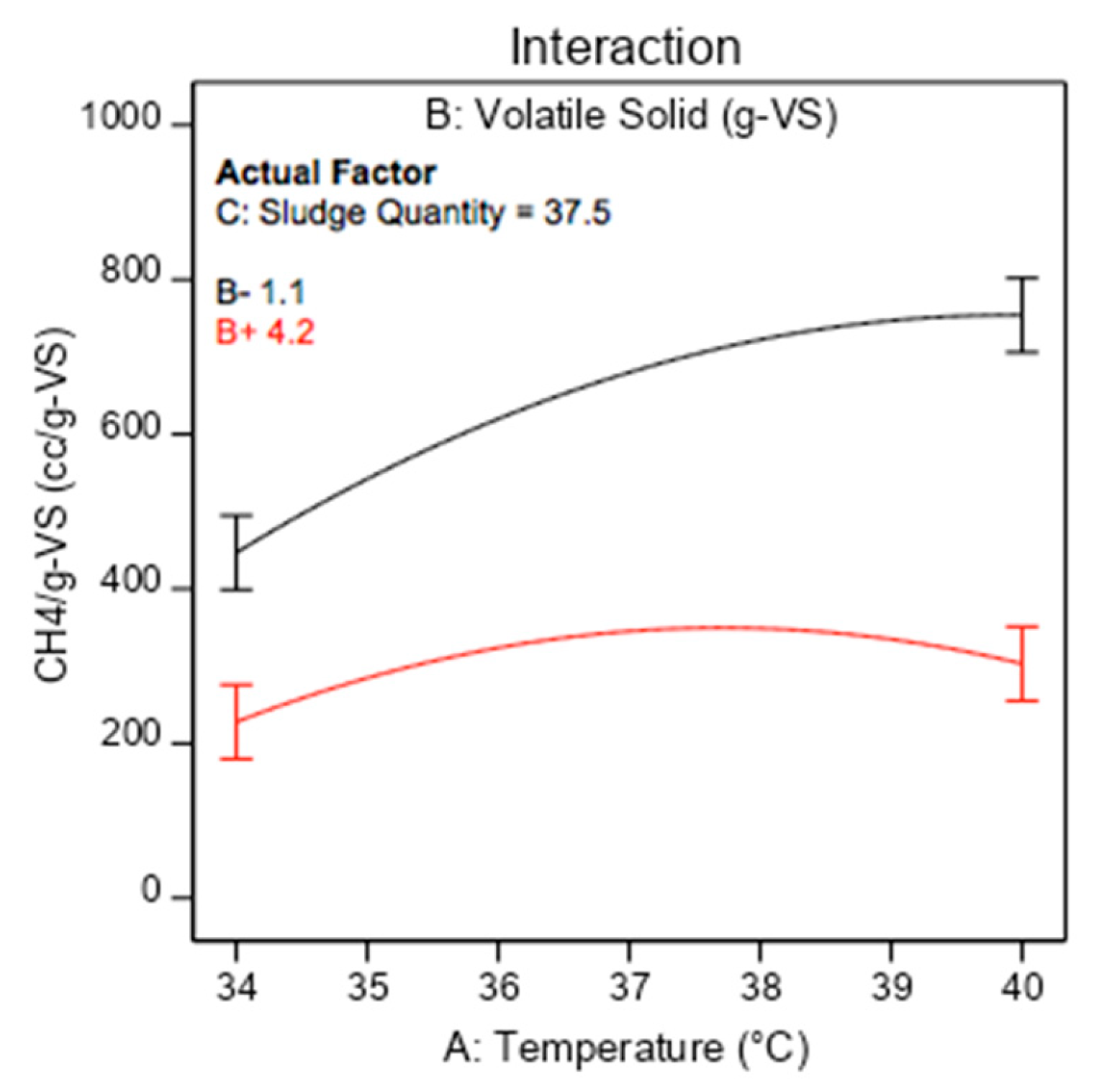
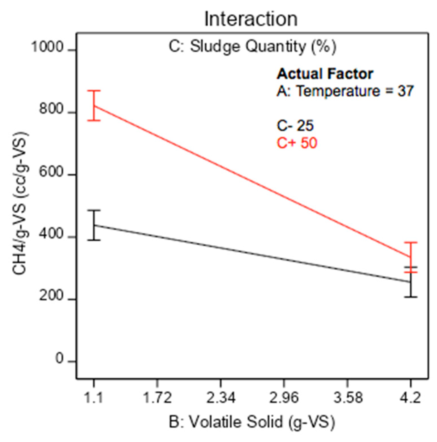
Figure 15 demonstrates the direct proportion between temperature and sludge quantity with CH4 g−1-VS. The volatile solid proportions indirectly with the methane g−1-VS, where at the lowest value of volatile solid of 1.1 g-VS, the highest methane g−1-VS was achieved, as illustrated in the same figure. The CH4 g−1-VS depends on its calculation by dividing it on the volatile solid value, so increasing the volatile solid value reduces the response value and vice versa. The influence of the interaction between the temperature and volatile solid is shown in Figure 16. The response doubled by increasing the temperature from 34 °C to 40 °C when using the volatile solid of 4.2 g-VS. While it slightly rise by increasing the temperature when using the volatile solid of 1.1g-VS. Figure 17 shows the effects of the interaction between the volatile solid and the sludge quantity. Also, the response doubled when the sludge quantity increases from 25% to 50% when using volatile solid of 1.1 g-VS. As shown in the same figure, the methane g−1-VS for both sludge quantities was at same value when the volatile solid value of 4.2 g-VS and this is due to the methane inhibition [32]. The contour plot that shown in Figure 18 clarifies that the highest CH4 g−1-VS resulted from volatile solids of 1.1 g-VS and a sludge quantity of 50%. As is clear from coded Equation (14), the volatile solid influence was the highest on the response:
CH4 g−1-VS = 512.58 + 95.59A − 167.42B + 115.84C-57.98AB − 76.13BC − 79.6A2 − 49.86C2
CH4 g−1-VS = −14,899.53404 + 719.50991 Temperature + 500.62903 Volatile Solid + 43.61388 Sludge Quantity 12.46774 Temperature × Volatile Solid − 3.92903 Volatile Solid × Sludge Quantity − 8.84605 Temperature2 − 0.319133 Sludge Quantity2
3.3.6. Digestate
Table 10 shows the content of the resulted digestate that constitute the three main nutrients of conventional fertilizers (N, P and K) and the dry matter. These amounts of nutrients match with what is recommended [33,34]. The presence of these elements in the resulted digestate enhances the possibility of its usage in different areas such as agriculture, whether in its liquid form or after its been dried.
3.4. Optimisation and Energy Evaluation
3.4.1. The optimisation
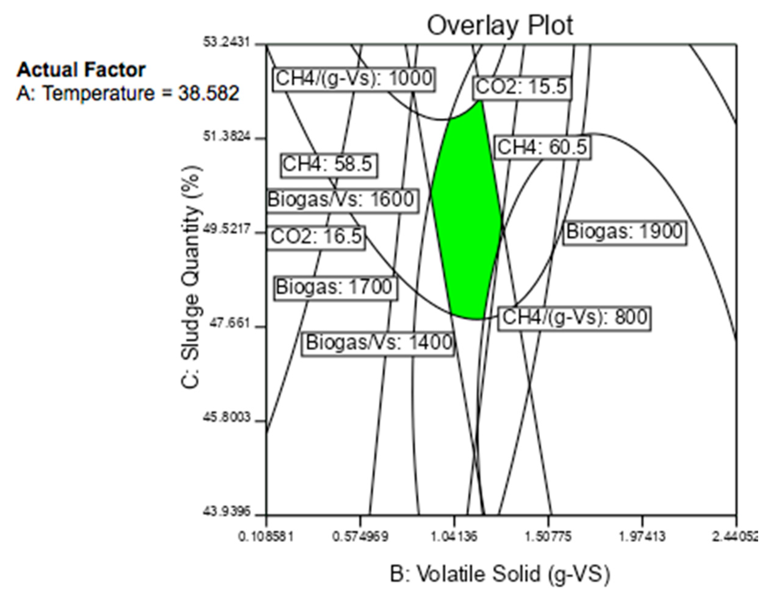
The optimisation process was carried out in the study for calculating the energy balance at the optimal results. The results of the energy balance may at a later time allow investigating the economic effect of the incorporation of the production process of starch-based products on the economic feasibility of the AD plants. The optimisation process was carried out in the study based on three criteria. The first criterion was set in terms of the quality with no limitation on the factors, while the other two were set in terms of cost. In all three criteria, the goals of the responses were fixed as follows: maximise the biogas g−1-VS, CH4%, CH4 g−1-VS and minimizing the CO2%. Due to the major influence of the concentration of CH4 on the value of the energy gained from a gram of volatile solid (Ep), the importance of the CH4% response was set to 5 (the highest) while the importance of the other responses were set to 3.
Furthermore, the gate fee is one of the main revenues of some AD plants [35]. Food processing industries are the second largest generator of wastes to the environment [36]. In addition to all of that, the maximisation of the volatile solid allows for benefiting from as much starch as possible and increases the contribution of the AD of CP in waste management. Therefore, the goal of the volatile solid factor was set to “maximise” in the 2nd and 3rd criteria.
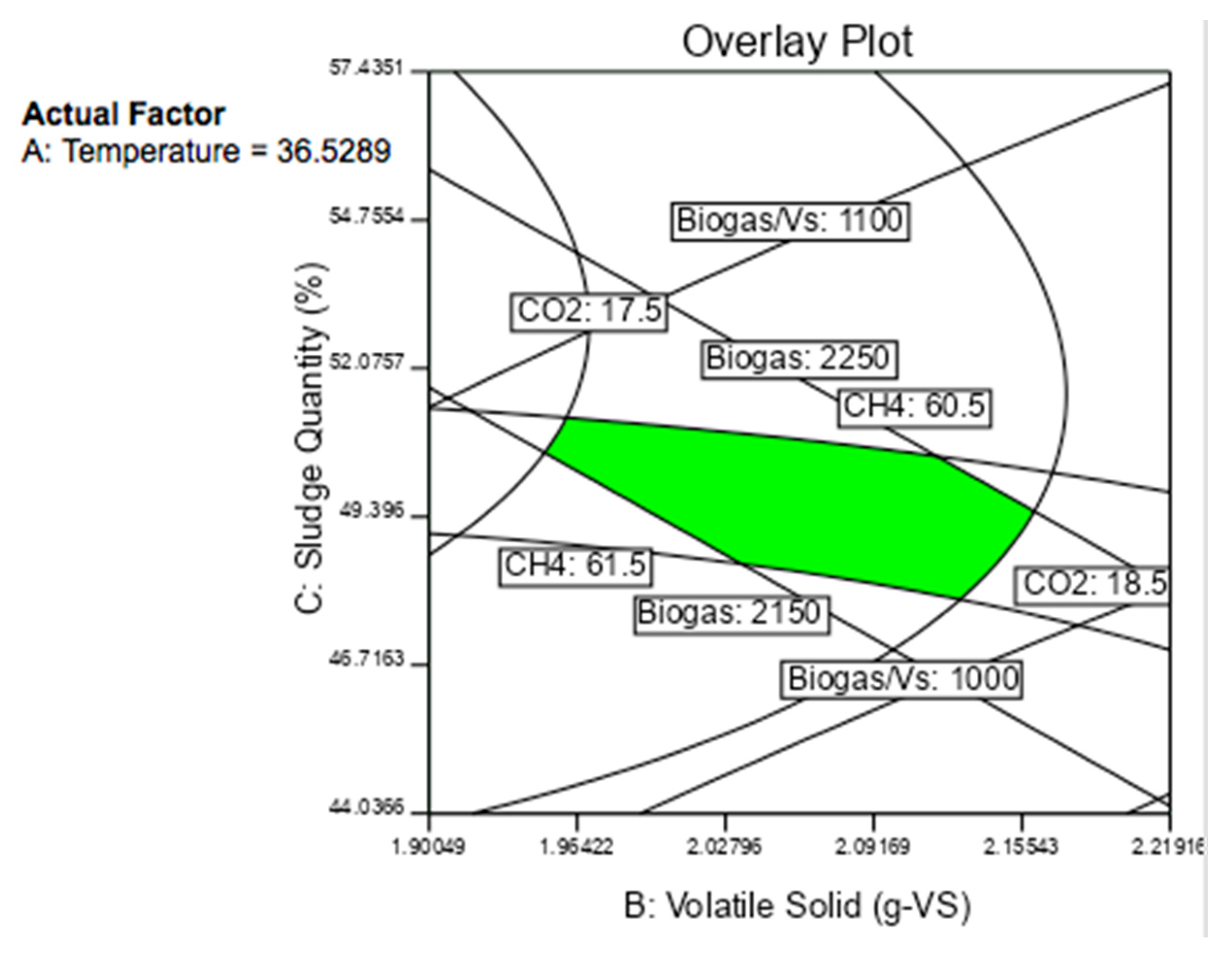
According to Cré—Composting and Anaerobic Digestion Association of Ireland [37]—sludge usually contains high proportions of water. The preservation of the digestate negatively influences the economic aspects of the AD plants [35,38]. As long as the AD plants are producing biogas, digestate will be generated. On one hand, the generation of the digestate in large amounts has a negative impact on the environment and could lead to major issues [39]. On the other hand, storing, transporting and maintaining the digestate in large amounts is costly as the TS of the digestate is usually low and its MS is high [35]. As a result the sludge quantity has a significant influence on the quantity and quality of the biogas produced from the AD of CP, its goal was set to “minimise” in the 2nd criterion. In the setting of the 3rd criterion, all these factors were taken into accounts in addition to the revenue of the AD plants from the sales of the biofertilizer and the goal of the sludge quantity was set to “in range”.
In terms of temperature, it was set to “minimise” in the 2nd and 3rd criteria in order to reduce the cost of the energy consumed in the digestion process. Note, however, the digestion process is a major expense for AD plants, whereas the energy consumed in the beating pre-treatment was quite low and thus neglected. Table 11 shows the three criteria and their goals. DOE provides the optimal results numerically and graphically.
3.4.2. Energy Evaluation
The insignificant influence of the starch on the biogas produced from the AD of the CP supports exploiting the starch as a raw material in the production of bio products simultaneously with the biogas and bio-slurry. The production of starch-based products simultaneously with biogas and bio-slurry could enhance the economic feasibility of AD plants.
Table 12 illustrates the optimal results based on the three criteria numerically. Figure 19, Figure 20 and Figure 21 show the optimal results at the optimal set of factors in over-lay figures based on each of the criterion. As shown in Table 12, the CH4% resulted from the three results were closer to each other. In terms of the biogas volume produced from the gram volatile solid, the highest volume was a result of the quality criteria (1st criterion) while, the lowest was based on the second criterion. The average electric energy consumed by the water baths at temperatures of 34, 37 and 40 °C were 50.54, 61.51 and 79.61 kWh, respectively.
Table 13 shows the energy gain/loss based on the optimal results. In the calculation of the energy balance, the optimal results that were selected by the software, as the highest in desirability, were the only ones considered. From the same table, it can be noted that the highest loss was attributed to the quality criterion while the highest energy gain was based on the 3rd criterion. As it is clear from that table, the changing of the goal of the sludge quantity from “minimise” to “in range” led to a 40% increase in the energy gain. On the other hand, the changing of the goals of the temperature and volatile solid concentration in the 1st and 3rd criterion to “minimise” and “maximise”, respectively, resulted in a large increase in the energy balance. This finding enhances the economic feasibility of the AD plants by reducing the energy consumed in the digestion process and applying gate fees for accepting wastes. The finding also supports increasing the contribution of the AD of CP in waste management.
4. Conclusions
The major findings of the study would support future investigations of the production of multiple starch-based bio-products alongside for biogas and bio-slurry applications. Compared to recent studies on the AD biogas of cassava peel, Hollander beater has been considered effective machinery to treat the CP and extracting the starch at the same time. Additionally, it has led to better results in terms of the quantity and quality of the biogas. The highest energy gain obtained was at the optimal result of 2195 cc biogas, 1053.2 cc g−1-VS. 60.9% CH4, 17.9% CO2 and 652.4 cc g−1-VS of methane at 36.5 °C, 2 g-VS and 200 mL of sludge. The biogas resulted from the 1st criterion is greater than that on the 2nd and 3rd criteria by 16.6% and 8.4% respectively. In terms of the highest methane g−1-VS yield based on the optimal results, the 1st criterion provided the highest methane g−1-VS volume of 871.5 cc g−1-VS which is 33.6% higher than 2nd criterion and 25% more than 3rd criterion. The results of the energy balance are supportive for AD plants for applying the gate fees for accepting the wastes and increasing the contribution of the AD of cassava peels on the waste management. The results of the tests based on the digestate application, confirmed its content to the three basic nutrients of fertilizer.
On the impact of starch from the biogas produced, it is considered quite low and findings have indicated its evaluations may enhance the economic feasibility of the AD to a greater extent. Therefore, future studies are recommended in analysing other factors, such as the retention time and the organic loading rate for certainty of the process.
The accumulation of the digestate post the AD process and the cost of maintaining the digestate are some of the major challenges for AD plants. Overcoming these challenges could enhance the sustainability of AD, hence, reducing the dependence on fossil fuel. Finding solutions for these challenges requires proposing studies to investigate the impact of the starch on the biogas produced from the CP by the AD process. This will test the potential of the digestate in serving as a bio-fertilizer since the economic feasibility of AD is strongly contingent on the biogas potential of the substrate. Higher biogas production from a given feedstock like CP will directly corresponds to shorter payback periods for commercial AD facilities based on the investment involved.
This study was carried out at the lab-scale and it shows good results. It is recommended to be performed in large-scale to assess its applicability on reality. It is also advisable to apply the study to other food wastes that contain starch and compare it with the results before extracting starch and with other related studies.
Author Contributions
The authors’ contributions are as follows. Conceptualization, methodology, writing—original draft preparation, software and data curation: A.M.A.; resources, software, formal analysis and data curation: R.A.; software, writing—review and editing, validation, visualization, formal analysis and investigation: K.Y.B.; project administration, validation, visualization, supervision and writing—review and editing: J.S. All authors have read and agreed to the published version of the manuscript.
Funding
This works was funded by Saudi Cultural Bureau in Dublin.
Acknowledgments
The author would like to thank the Green Generation Plants, Kildare in Ireland in the provision of sludge for the experimental work in this study. The author with thanks gratefully acknowledges the financial support provided by the Ministry of Education of the Kingdom of Saudi Arabia represented by the Saudi Cultural Bureau in Ireland.
Conflicts of Interest
The authors declare no conflict of interest.
Nomenclature
| AD | Anaerobic digestion |
| N | Nitrogen |
| P | Phosphorous |
| K | Potassium |
| DOE | Design of experiment |
| RSM | Response surface methodology |
| Significance level | |
| CP | Cassava peel |
| VS | Volatile Solid |
| TS | Total solid |
| MS | Moisture content |
| SQ | Sludge quantity |
| ANOVA | Analysis of variance |
| BBD | Box-Behnken design |
| Pred. R2 | Predicted R2 |
| Adj. R2 | Adjusted R2 |
| Adeq. Precision | Adequate Precision |
| Cor total | Total sum of the squares corrected for the mean |
| df | Degree of freedom |
| Bs | The energy content of biogas produced by CP in [kW h/m3] |
| 9.67 | The energy content of 1 Nm3 (Normal cubic meter) of biogas. |
| Ep | The energy gained from a gram of volatile solid of CP from the biogas produced in [Wh g−1-VS] |
| Bp | The biogas volume produced from each gram of volatile solid of CP. |
| Ec | The energy consumed by the water bath to digest the gram volatile solid of CP in [Wh g−1-VS]. |
| Ept | The electric energy consumed in the digestion process, which was measured by a prodigit kilowatt-hour meter. |
| VSm | The total amount of volatile solid in the water bath |
| Net Ep | The net energy produced by a gram of volatile solid of treated CP in [Wh g−1-VS] |
References
- Paepatung, N.; Nopharatana, A.; Songkasiri, W. Bio-Methane Potential of Biological Solid Materials and Agricultural Wastes. Asian J. Energy Environ. 2009, 10, 19–27. [Google Scholar]
- Guo, X.; Wang, C.; Sun, F.; Zhu, W.; Wu, W. A comparison of microbial characteristics between the thermophilic and mesophilic anaerobic digesters exposed to elevated food waste loadings. Bioresour. Technol. 2014, 152, 420–428. [Google Scholar] [CrossRef] [PubMed]
- FAO. Food Wastage Footprint Impacts on Natural Resources; Food and Agriculture Organisation of the United Nations—FAO: Rome, Italy, 2013. [Google Scholar]
- The World Bank. Total Greenhouse Gas Emissions (Kt of CO2 Equivalent). 2016. Available online: data.worldbank.org/indicator/EN.ATM.GHGT.KT.CE (accessed on 26 February 2019).
- Slorach, P.C.; Jeswani, H.K.; Cuéllar-Franca, R.; Azapagic, A. Environmental sustainability of anaerobic digestion of household food waste. J. Environ. Manag. 2019, 236, 798–814. [Google Scholar] [CrossRef] [PubMed]
- Teixeira, E.; Pasquini, D.; Curvelo, A.; Corradini, E.; Belgacem, M.; Dufresne, A. Cassava bagasse cellulose nanofibrils reinforced thermoplastic cassava starch. Carbohydr. Polym. 2009, 87, 422–431. [Google Scholar] [CrossRef]
- Ghimire, A.; Sen, R.; Annachhatre, A. Biosolid Management Options in Cassava Starch Industries of Thailand: Present Practice and Future Possibilities. Procedia Chem. 2015, 14, 66–75. [Google Scholar] [CrossRef] [Green Version]
- Sawyerr, N.; Trois, N.; Workneh, T.; Okudoh, V. Co-Digestion of Animal Manure and Cassava Peel for Biogas Production in South Africa. In Proceedings of the 9th Int’l Conference on Advances in Science, Engineering, Technology & Waste Management (ASETWM-17), Parys, South Africa, 27–28 November 2017; pp. 101–106. [Google Scholar]
- Sivamani, S.; Chandrasekaran, A.; Balajii, M.; Shanmugaprakash, M. Evaluation of the potential of cassava-based residues for biofuels production. Rev. Environ. Sci. Bio/Technol. 2018, 17, 553–570. [Google Scholar] [CrossRef]
- Iyayi, E.; Losei, D. Protein Enrichment of Cassava By-products Through Solid State Fermentation By Fungi. J. Food Technol. Afr. 2001, 6, 116–118. [Google Scholar] [CrossRef] [Green Version]
- Aro, S.; Aletor, V.; Tewe, O.; Agbede, J. Nutritional potentials of cassava tuber wastes: A case study of a cassava starch processing factory in south-western Nigeria. Livest. Res. Rural Dev. 2010, 22, 42–47. [Google Scholar]
- Obadina, O.; Oyewole, B.; Sanni, O.; Abiola, S. Fungal enrichment of cassava peels proteins. Afr. J. Biotechnol. 2006, 5, 302–304. [Google Scholar]
- Ezekiel, O.; Aworh, O. Simultaneous saccharification and cultivation of Candida utilis on cassava peel. Innov. Food Sci. Emerg. Technol. 2018, 49, 184–191. [Google Scholar] [CrossRef]
- Okoroigw, E.; Ofomatah, A.; Oparaku, N. Biodigestion of cassava peels blended with pig dung for methane generation. Afr. J. Biotechnol. 2013, 12, 5956–5961. [Google Scholar]
- Andréa, L.; Paussb, A.; Ribeiro, T. Solid anaerobic digestion: State-of-art, scientific and technological hurdles. Bioresour. Technol. 2018, 247, 1027–1037. [Google Scholar] [CrossRef] [PubMed]
- Chen, Y.; Cheng, J.; Creamer, K. Inhibition of anaerobic digestion process: A review. Bioresour. Technol. 2008, 99, 4044–4064. [Google Scholar] [CrossRef] [PubMed]
- Li, Y.; Park, S.; Zhu, J. Solid-state anaerobic digestion for methane production from organic waste. Renew. Sustain. Energy Rev. 2011, 15, 821–826. [Google Scholar] [CrossRef]
- Tippayawong, N.; Thanompongchart, P. Biogas quality upgrade by simultaneous removal of CO2 and H2S in a packed column reactor. Energy 2010, 35, 4531–4535. [Google Scholar] [CrossRef]
- Rapport, J.; Zhang, R.; Jenkins, B.M.; Williams, R.B. Current Anaerobic Digestion Technologies Used for Treatment of Municipal Organic Solid Waste; California Environmental Protection Agency: Sacramento, CA, USA, 2008. [Google Scholar]
- Jekayinfa, S.; Scholz, V. Laboratory Scale Preparation of Biogas from Cassava Tubers, Cassava Peels, and Palm Kernel Oil Residues. Energy Sources Part. A Recovery Util. Environ. Eff. 2013, 35, 2022–2032. [Google Scholar] [CrossRef]
- Nkodi, T.; Taba, K.; Sungula, J.; Mulaji, C.; Mihigo, S. Biogas Production by Co-Digestion of Cassava Peels with Urea. Int. J. Sci. Eng. Technol. 2016, 5, 139–141. [Google Scholar]
- Zhang, J.; Xu, J.; Wang, D.; Ren, N. Anaerobic Digestion of Cassava Pulp with Sewage Sludge Inocula. BioResources 2016, 11, 451–465. [Google Scholar] [CrossRef]
- Panichnumsin, P.; Nopharatana, A.; Ahring, B.; Chaiprasert, P. Production of methane by co-digestion of cassava pulp with various concentrations of pig manure. Biomass Bioenergy 2010, 34, 1117–1124. [Google Scholar] [CrossRef]
- Glanpracha, N.; Annachhatre, A.P. Anaerobic co-digestion of cyanide containing cassava pulp with pig manure. Bioresour. Technol. 2016, 214, 112–121. [Google Scholar] [CrossRef]
- Montingelli, M.; Benyounis, K.; Quilty, B.; Stokes, J.; Olabi, A. Influence of mechanical pretreatment and organic concentration of Irish brown seaweed for methane production. Energy 2017, 118, 1079–1089. [Google Scholar] [CrossRef] [Green Version]
- Logan, M.; Safi, M.; Lens, P.; Visvanathan, C. Investigating the performance of internet of things based anaerobic digestion of food waste. Process. Saf. Environ. Prot. 2019, 127, 277–287. [Google Scholar] [CrossRef]
- Montingelli, M.; Benyounis, K.; Stokes, J.; Olabi, A. Pretreatment of macroalgal biomass for biogas production. Energy Convers. Manag. 2016, 108, 202–209. [Google Scholar] [CrossRef]
- Adekunle, A.; Orsat, V.; Raghavan, V. Lignocellulosic bioethanol: A review and design conceptualization study of production from cassava peels. Renew. Sustain. Energy Rev. 2018, 64, 518–531. [Google Scholar] [CrossRef]
- Sivamania, S.; Archanaa, K.; Santhosha, R.; Sivarajasekara, N.; Prasad, N. Synthesis and characterization of starch nanoparticles from cassava Peel. J. Bioresour. Bio-Prod. 2018, 3, 161–165. [Google Scholar]
- Toreci, I.; Droste, R.L.; Kennedy, K.J. Mesophilic Anaerobic Digestion with High-Temperature Microwave Pretreatment and Importance of Inoculum Acclimation. Water Environ. Res. 2011, 83, 549–559. [Google Scholar] [CrossRef]
- Wilkins, D.; Rao, S.; Lu, X.; Lee, P. Effects of sludge inoculum and organic feedstock on active microbial communities and methane yield during anaerobic digestion. Front. Microbiol. 2015, 13, 1114. [Google Scholar] [CrossRef] [Green Version]
- Srisowmeya, G.; Chakravarthy, M.; Devi, G.N. Critical considerations in two-stage anaerobic digestion of food waste–A review. Renew. Sustain. Energy Rev. 2019, 1, 109587. [Google Scholar] [CrossRef]
- Alrefai, R.; Benyounis, K.; Stokes, J. Integration approach of anaerobic digestion and fermentation process towards producing biogas and bioethanol with zero waste: Technical. J. Fundam. Renew. Energy Appl. 2017, 7, 243. [Google Scholar] [CrossRef]
- The Official Information Portal on Anaerobic Digestion. Available online: http://www.biogas-info.co.uk/about/digestate/ (accessed on 7 January 2020).
- Mouat, A.; Barclay, A.; Mistry, P.; Webb, J. Digestate Market. Development in Scotland; Scottish Government: Edinburgh, UK, 2010.
- Gowe, C. Review on Potential Use of Fruit and Vegetables By-Products as A Valuable Source of Natural Food Additives. Food Sci. Qual. Manag. 2015, 45, 47–61. [Google Scholar]
- McDonnell, D.; Burke, M.; Dowdall, J.; Foster, P.; Mahon, K. Guidelines for Anaerobic Digestion in Ireland. 2018. Available online: http://www.cre.ie/web/wp-content/uploads/2018/03/Guidelines-for-Anaerobic-Digestion-in-Ireland_Final.pdf (accessed on 19 March 2019).
- Plana, P.V.; Noche, B. A Review of the Current Digestate Distribution Models: Storage and Transport. WIT Trans. Ecol. Environ. 2016, 202, 345–357. [Google Scholar]
- Wang, D.; Xi, J.; Ai, P.; Yu, L.; Zhai, H.; Yan, S.; Zhang, Y. Enhancing ethanol production from thermophilic and mesophilic solid digestate using ozone combined with aqueous ammonia pretreatment. Bioresour. Technol. 2016, 207, 52–58. [Google Scholar] [CrossRef] [PubMed]
Figure 1.
The flowchart of the experiment.

Figure 2.
Normal probability and predicted vs. actual residual plots of biogas produced from CP.

Figure 3.
Normal probability and predicted vs. actual residual plots of CH4% produced from CP.

Figure 4.
Perturbation plot shows the effect of all factors on the biogas volume.

Figure 5.
Contour plot views the effect of temperature and volatile solid on the Biogas volume at sludge quantity of 37.5%.
Figure 5.
Contour plot views the effect of temperature and volatile solid on the Biogas volume at sludge quantity of 37.5%.

Figure 6.
Perturbation plot shows the effect of all factors on the biogas g−1-VS volume.

Figure 7.
Interaction plot clarifies the effect of interaction between temperature and volatile solid on biogas g−1-VS.
Figure 7.
Interaction plot clarifies the effect of interaction between temperature and volatile solid on biogas g−1-VS.

Figure 8.
Contour plot views the effect of temperature and volatile solid on the biogas g−1-VS volume at sludge quantity of 37.5%.
Figure 8.
Contour plot views the effect of temperature and volatile solid on the biogas g−1-VS volume at sludge quantity of 37.5%.

Figure 9.
Perturbation plot showing the effect of all factors on CH4%.

Figure 10.
Interaction plot clarifying the effect of interaction between volatile solid and sludge quantity on CH4%.
Figure 10.
Interaction plot clarifying the effect of interaction between volatile solid and sludge quantity on CH4%.

Figure 11.
Contour plot showing the effect of volatile solid and sludge quantity on the CH4% volume at temperature of 37 °C.
Figure 11.
Contour plot showing the effect of volatile solid and sludge quantity on the CH4% volume at temperature of 37 °C.

Figure 12.
Perturbation plot showing the effect of all factors on the CO2%.

Figure 13.
Interaction plot clarifying the effect of interaction between volatile solid and sludge quantity on CO2%.
Figure 13.
Interaction plot clarifying the effect of interaction between volatile solid and sludge quantity on CO2%.

Figure 14.
Contour plot showing the effect of volatile solid and sludge quantity on the CO2% volume at temperature of 37 °C.
Figure 14.
Contour plot showing the effect of volatile solid and sludge quantity on the CO2% volume at temperature of 37 °C.

Figure 15.
Perturbation plot showing the effect of all factors on the CH4 g−1-VS.

Figure 16.
Interaction plot displaying the effects of interaction between temperature and volatile solid on CH4 g−1-VS.
Figure 16.
Interaction plot displaying the effects of interaction between temperature and volatile solid on CH4 g−1-VS.

Figure 17.
Interaction plot clarifying the effects of interaction between volatile solid and sludge quantity on CH4 g−1-VS.
Figure 17.
Interaction plot clarifying the effects of interaction between volatile solid and sludge quantity on CH4 g−1-VS.

Figure 18.
Contour plot showing the effect of volatile solid and sludge quantity on the CH4 g−1-VS% at a temperature of 37 °C.
Figure 18.
Contour plot showing the effect of volatile solid and sludge quantity on the CH4 g−1-VS% at a temperature of 37 °C.

Figure 19.
Overlay plot based on the first criterion.

Figure 20.
Overlay plot based on the second criterion.

Figure 21.
Overlay plot based on the third criterion.


Table 1.
Variable matrix and levels in actual values.
| Factors and Their Codes | Unit | Lower Level | Centre Point | Upper Level |
|---|---|---|---|---|
| Temperature (A) | °C | 34 | 37 | 40 |
| Volatile Solid (B) | g-VS | 1.1 | 2.65 | 4.2 |
| Sludge Quantity (C) | % | 25 | 37.5 | 50 |
Table 2.
Control sample conditions.
| Sample No. | Factor 1 | Factor 2 | Factor 3 |
|---|---|---|---|
| A: Temperature | B: Volatile Solid | C: Sludge Quantity | |
| °C | g-VS | % | |
| 1 | 34 | 4.0 | 50 |
| 2 | 37 | 4.0 | 50 |
| 3 | 40 | 4.0 | 50 |
Table 3.
The experiment responses results.
| Std. | Run | Factor 1 | Factor 2 | Factor 3 | Resp.1 | Resp.2 | Resp.3 | Resp. 4 | Resp.5 |
|---|---|---|---|---|---|---|---|---|---|
| A | B | C | Biogas | Biogas g−1-VS | CH4 | CO2 | CH4g−1-VS | ||
| °C | g-VS | % | cc | cc g−1-VS | % | % | cc g−1-VS | ||
| 1 | 10 | 34 | 1.1 | 37.5 | 831 | 755.4 | 56.8 | 19.6 | 428.8 |
| 2 | 7 | 40 | 1.1 | 37.5 | 1587 | 1442.5 | 54.5 | 21 | 786.7 |
| 3 | 9 | 34 | 4.2 | 37.5 | 2275 | 541.7 | 39.7 | 36.1 | 214.9 |
| 4 | 1 | 40 | 4.2 | 37.5 | 3367 | 801.6 | 42.5 | 33.7 | 340.9 |
| 5 | 12 | 34 | 2.65 | 25 | 1271 | 479.7 | 45.8 | 29.2 | 219.8 |
| 6 | 4 | 40 | 2.65 | 25 | 1844 | 695.8 | 47.1 | 28.3 | 327.7 |
| 7 | 8 | 34 | 2.65 | 50 | 1870 | 705.7 | 54.7 | 22.5 | 386.3 |
| 8 | 5 | 40 | 2.65 | 50 | 2562 | 966.9 | 57.8 | 20.4 | 559.2 |
| 9 | 6 | 37 | 1.1 | 25 | 1096 | 996 | 43.6 | 32 | 434.2 |
| 10 | 14 | 37 | 4.2 | 25 | 3064 | 729.5 | 33.8 | 37.8 | 246.6 |
| 11 | 16 | 37 | 1.1 | 50 | 1552 | 1411 | 60.3 | 15.9 | 850.8 |
| 12 | 17 | 37 | 4.2 | 50 | 3830 | 911.9 | 39.3 | 35.7 | 358.7 |
| 13 | 11 | 37 | 2.65 | 37.5 | 2390 | 928.2 | 58.3 | 23.4 | 540.8 |
| 14 | 3 | 37 | 2.65 | 37.5 | 2169 | 818.6 | 59.8 | 22.9 | 489.8 |
| 15 | 15 | 37 | 2.65 | 37.5 | 2210 | 833.8 | 61.8 | 22.7 | 515 |
| 16 | 2 | 37 | 2.65 | 37.5 | 2255 | 851 | 58.5 | 24.6 | 497.5 |
| 17 | 13 | 37 | 2.65 | 37.5 | 2225 | 839.5 | 57.2 | 22.5 | 480.4 |
Table 4.
Comparison between actual and predicted values of control samples.
| Resp. | Control Samples | Predicted Value | ||||||||
|---|---|---|---|---|---|---|---|---|---|---|
| Biogas | Biogas g−1-VS | CH4 | CO2 | CH4 g−1-VS | Biogas | Biogas g−1-VS | CH4 | CO2 | CH4 g−1-VS | |
| Unit | cc | cc g−1-VS | % | % | cc g−1-VS | cc | cc g−1-VS | % | % | cc g−1-VS |
| 1 | 2766.1 | 691.5 | 40.5 | 35.0 | 280.1 | 2727.7 | 667.3 | 40.2 | 35.2 | 243.0 |
| 2 | 3558.7 | 889.7 | 42.9 | 33.3 | 381.4 | 3479.2 | 882.8 | 42.7 | 33.9 | 365.2 |
| 3 | 3630.5 | 907.6 | 41.7 | 32.3 | 378.8 | 3505.9 | 837.3 | 41.5 | 32.6 | 333.2 |
Table 5.
ANOVA table for the biogas response.
| Source | Sum of Squares | df | Mean Square | F-Value | p-Value | |
|---|---|---|---|---|---|---|
| Model | 9.539 × 10⁶ | 4 | 2.385 × 10⁶ | 86.14 | <0.0001 | Significant |
| A-Temperature | 1.211 × 10⁶ | 1 | 1.211 × 10⁶ | 43.76 | <0.0001 | |
| B-Volatile Solid | 6.975 × 10⁶ | 1 | 6.975 × 10⁶ | 251.97 | <0.0001 | |
| C-Sludge Quantity | 8.058 × 10⁵ | 1 | 8.058 × 10⁵ | 29.11 | 0.0002 | |
| A2 | 5.466 × 10⁵ | 1 | 5.466 × 10⁵ | 19.74 | 0.0008 | |
| Residual | 3.322 × 10⁵ | 12 | 27,682.67 | |||
| Lack of Fit | 3.038 × 10⁵ | 8 | 37,972.65 | 5.35 | 0.0614 | Not significant |
| Pure Error | 28,410.80 | 4 | 7102.70 | |||
| Cor Total | 9.871 × 10⁶ | 16 | ||||
| Adequacy measuring tools | R2 = 0.9663 | Adjusted R2 = 0.9551 | Predicted R2 = 0.9212 | |||
Table 6.
ANOVA table for biogas g−1-VS response.
| Source | Sum of Squares | df | Mean Square | F-Value | p-Value | |
|---|---|---|---|---|---|---|
| Model | 9.592 × 10⁵ | 6 | 1.599 × 10⁵ | 31.05 | <0.0001 | Significant |
| A-Temperature | 2.536 × 10⁵ | 1 | 2.536 × 10⁵ | 49.24 | <0.0001 | |
| B-Volatile Solid | 3.281 × 10⁵ | 1 | 3.281 × 10⁵ | 63.72 | <0.0001 | |
| C-Sludge Quantity | 1.497 × 10⁵ | 1 | 1.497 × 10⁵ | 29.08 | 0.0003 | |
| AB | 45,624.96 | 1 | 45,624.96 | 8.86 | 0.0139 | |
| A2 | 76,839.04 | 1 | 76,839.04 | 14.92 | 0.0031 | |
| B2 | 1.152 × 10⁵ | 1 | 1.152 × 10⁵ | 22.37 | 0.0008 | |
| Residual | 51,494.42 | 10 | 5149.44 | |||
| Lack of Fit | 44,108.57 | 6 | 7351.43 | 3.98 | 0.1011 | Not significant |
| Pure Error | 7385.85 | 4 | 1846.46 | |||
| Cor Total | 1.011 × 10⁶ | 16 | ||||
| Adequacy measuring tools | R2 = 0.9491 | Adjusted R2 = 0.9185 | Predicted R2 = 0.7554 | |||
Table 7.
ANOVA table for CH4% response.
| Source | Sum of Squares | df | Mean Square | F-Value | p-Value | |
|---|---|---|---|---|---|---|
| Model | 1240.05 | 7 | 177.15 | 69.90 | <0.0001 | Significant |
| A-Temperature | 3.00 | 1 | 3.00 | 1.18 | 0.3048 | |
| B-Volatile Solid | 448.50 | 1 | 448.50 | 176.98 | <0.0001 | |
| C-Sludge Quantity | 218.40 | 1 | 218.40 | 86.18 | <0.0001 | |
| BC | 31.36 | 1 | 31.36 | 12.37 | 0.0065 | |
| A2 | 13.99 | 1 | 13.99 | 5.52 | 0.0434 | |
| B2 | 335.20 | 1 | 335.20 | 132.27 | <0.0001 | |
| C2 | 148.94 | 1 | 148.94 | 58.77 | <0.0001 | |
| Residual | 22.81 | 9 | 2.53 | |||
| Lack of Fit | 10.42 | 5 | 2.08 | 0.6729 | 0.6674 | Not significant |
| Pure Error | 12.39 | 4 | 3.10 | |||
| Cor Total | 1262.86 | 16 | ||||
| Adequacy measuring tools | R2 = 0.9819 | Adjusted R2 = 0.9679 | Predicted R2 = 0.9459 | |||
Table 8.
ANOVA table for CO2% response.
| Source | Sum of Squares | df | Mean Square | F-Value | p-Value | |
|---|---|---|---|---|---|---|
| Model | 689.15 | 7 | 98.45 | 114.70 | <0.0001 | Significant |
| A-Temperature | 2.00 | 1 | 2.00 | 2.33 | 0.1612 | |
| B-Volatile Solid | 375.38 | 1 | 375.38 | 437.35 | <0.0001 | |
| C-Sludge Quantity | 134.48 | 1 | 134.48 | 156.68 | <0.0001 | |
| AB | 3.61 | 1 | 3.61 | 4.21 | 0.0705 | |
| BC | 49.00 | 1 | 49.00 | 57.09 | <0.0001 | |
| B2 | 96.96 | 1 | 96.96 | 112.97 | <0.0001 | |
| C2 | 22.18 | 1 | 22.18 | 25.84 | 0.0007 | |
| Residual | 7.72 | 9 | 0.8583 | |||
| Lack of Fit | 4.90 | 5 | 0.9793 | 1.39 | 0.3873 | Not significant |
| Pure Error | 2.83 | 4 | 0.7070 | |||
| Cor Total | 696.88 | 16 | ||||
| Adequacy measuring tools | R2 = 0.9889 | Adjusted R2 = 0.9803 | Predicted R2 = 0.942 | |||
Table 9.
ANOVA table for CH4 g−1-VS response.
| Source | Sum of Squares | df | Mean Square | F-Value | p-Value | |
|---|---|---|---|---|---|---|
| Model | 4.806 × 10⁵ | 7 | 68,651.47 | 50.86 | <0.0001 | Significant |
| A-Temperature | 73,095.76 | 1 | 73,095.76 | 54.16 | <0.0001 | |
| B-Volatile Solid | 2.242 × 10⁵ | 1 | 2.242 × 10⁵ | 166.14 | <0.0001 | |
| C-Sludge Quantity | 1.073 × 10⁵ | 1 | 1.073 × 10⁵ | 79.53 | <0.0001 | |
| AB | 13,444.40 | 1 | 13,444.40 | 9.96 | 0.0116 | |
| BC | 23,180.06 | 1 | 23,180.06 | 17.17 | 0.0025 | |
| A2 | 26,762.41 | 1 | 26,762.41 | 19.83 | 0.0016 | |
| C2 | 10,498.41 | 1 | 10,498.41 | 7.78 | 0.0211 | |
| Residual | 12,147.72 | 9 | 1349.75 | |||
| Lack of Fit | 9874.08 | 5 | 1974.82 | 3.47 | 0.1256 | Not significant |
| Pure Error | 2273.64 | 4 | 568.41 | |||
| Cor Total | 4.927 × 10⁵ | 16 | ||||
| Adequacy measuring tools | R2 = 0.9753 | Adjusted R2 = 0.9562 | Predicted R2 = 0.8693 | |||
Table 10.
The results of the tests of the resulted digestate.
| Test | Unit | Result |
|---|---|---|
| Total phosphorous | mg/kg | 632 |
| Potassium | mg/kg | 526 |
| Total nitrogen | g/100g | 3886 |
| Dry matter | mg/kg | 2.7 |
Table 11.
The optimisation criterion and goals.
| Factors and Responses | 1st Criteria | 2nd Criteria | 3rd Criteria | |||
|---|---|---|---|---|---|---|
| Goal | Importance | Goal | Importance | Goal | Importance | |
| A: Temperature | In range | 3 | Minimise | 3 | Minimise | 3 |
| B: Volatile Solid | In range | 3 | Maximise | 3 | Maximise | 3 |
| C: Sludge Quantity | In range | 3 | Minimise | 3 | In range | 3 |
| Biogas | In range | 3 | In range | 3 | In range | 3 |
| Biogas g−1VS | Maximise | 3 | Maximise | 3 | Maximise | 3 |
| CH4 | Maximise | 5 | Maximise | 5 | Maximise | 5 |
| CO2 | Minimise | 3 | Minimise | 3 | Minimise | 3 |
| CH4 g−1VS | Maximise | 3 | Maximise | 3 | Maximise | 3 |
Table 12.
The optimal results of the three criteria.
| Criterion | A: °C | B: g-VS | C: % | Biogas cc | Biogas cc g−1-VS | CH4 % | CO2 % | CH4 g−1VS cc g−1-VS |
|---|---|---|---|---|---|---|---|---|
| 1st | 38.6 | 1.2 | 50.0 | 1831 | 1448.1 | 59.8 | 15.9 | 871.5 |
| 2nd | 36.8 | 2.1 | 39.4 | 2012 | 939.7 | 61.4 | 20.6 | 578.9 |
| 3rd | 36.5 | 2.0 | 50.0 | 2195.4 | 1053.2 | 60.9 | 17.9 | 652.4 |
Table 13.
Energy evaluation of the optimisation criterion.
| Criterion | Energy Nonsumed, kWh | VolAtile Solid Weight, g | Bs, kWh/m3 | Ep, kWh g−1-VS | Ec, kWh g−1-VS | Net Ep, kWh g−1-VS | Energy Balance,% |
|---|---|---|---|---|---|---|---|
| 1st | 70.6 | 1.15 | 5.78 | 0.62 | 0.82 | −0.20 | −23.27% |
| 2nd | 56.2 | 2.13 | 5.93 | 0.41 | 0.35 | 0.07 | 18.93% |
| 3rd | 56.2 | 2.05 | 5.89 | 0.47 | 0.37 | 0.10 | 27.26% |
© 2020 by the authors. Licensee MDPI, Basel, Switzerland. This article is an open access article distributed under the terms and conditions of the Creative Commons Attribution (CC BY) license (http://creativecommons.org/licenses/by/4.0/).
Share and Cite
MDPI and ACS Style
Alrefai, A.M.; Alrefai, R.; Benyounis, K.Y.; Stokes, J. Impact of Starch from Cassava Peel on Biogas Produced through the Anaerobic Digestion Process. Energies 2020, 13, 2713. https://doi.org/10.3390/en13112713
AMA Style
Alrefai AM, Alrefai R, Benyounis KY, Stokes J. Impact of Starch from Cassava Peel on Biogas Produced through the Anaerobic Digestion Process. Energies. 2020; 13(11):2713. https://doi.org/10.3390/en13112713
Chicago/Turabian StyleAlrefai, Alla Mohammed, Raid Alrefai, Khaled Younis Benyounis, and Joseph Stokes. 2020. "Impact of Starch from Cassava Peel on Biogas Produced through the Anaerobic Digestion Process" Energies 13, no. 11: 2713. https://doi.org/10.3390/en13112713
Note that from the first issue of 2016, this journal uses article numbers instead of page numbers. See further details here.